

Intermediate Physics for Medicine and Biology - Russell K. Hobbie & Bradley J. Roth
.pdf4.10 Example: Steady-State Di usion to a Spherical Cell and End E ects |
95 |
FIGURE 4.16. Di usive end e ects for a spherical cell pierced by pores.
simultaneously to relate i to concentrations C1 and C4:
|
πR2 |
D |
|
|
|
i = |
p |
|
(C1 |
− C4). |
(4.45) |
∆Z + 2πRp/4 |
|||||
This has the same form as Eq. 4.42, except that the membrane thickness has been replaced by an e ective thickness
∆Z = ∆Z + 2 |
πRp |
. |
(4.46) |
|
4 |
||||
|
|
|
An extra length πRp/4 has been added at each end to correct for di usion in the unstirred layer on each side of the pore. This correction is important when the pore length is less than two or three times the pore radius.
Now consider di usion in or out of the spherical cell shown in Fig. 4.16. The radius of the cell is B. The membrane has thickness ∆Z and is pierced by a total of N pores, each of radius Rp. Within the cell we do not know the details of the concentration distribution, since they depend on what sort of chemical reactions are taking place and where. But we will assume that at the radius where di usion to the pores becomes important, the concentration is C1. At the inner face of each pore it is C2, at the outer face it is C3, and over an approximately spherical surface of radius B it is C4. Far away, the concentration is C5. As a result, there are four separate regions in which we must consider di usion. The first is from C1 to the opening of each pore; the second is through the pore; third, there is di usion from the outer face of each pore to C4; and, finally, there is di usion from the spherical object of radius B to the surrounding medium.
where ∆Z is given by Eq. 4.46. Since there are N pores in all, the total flow through the cell wall is
|
N πR2 |
D |
|
|
icell = N ipore = |
p |
|
(C1 − C4). |
(4.48) |
∆Z |
|
|||
The di usion from C4 to infinity is given by Eq. 4.38c.
icell = 4πD B (C4 − C5), |
(4.49) |
where B is the e ective radius for di usion to the surrounding medium. It is slightly larger than B. If we equate Eqs. 4.48 and 4.49, solve for C4 and substitute this result back in Eq. 4.49, we get
icell = |
4πDB N Rp2 |
|
(C1 − C5). |
|
(4.50) |
||||||
N R2 + 4B |
∆Z |
|
|
||||||||
|
p |
|
|
|
|
|
|
|
|
|
|
This can be rewritten as |
|
|
|
|
|
|
|
|
|
||
|
|
N πR2D |
|
|
|
|
|
|
|
||
icell = |
|
p |
(C1 |
− C5), |
|
(4.51) |
|||||
∆Ze |
|
||||||||||
where |
|
|
|
|
|
|
|
Rp2 |
|
|
|
∆Ze = ∆Z + 2 |
πRp |
+ N |
. |
(4.52) |
|||||||
|
4 |
|
|
||||||||
|
|
|
|
|
|
4B |
|
|
|||
The first term in ∆Ze is the membrane thickness. The second term corrects for di usion from the end of each pore to the surrounding fluid; the last corrects for diffusion away from the cell into the surrounding medium. The third term can be expressed as
N Rp2 = B Bf,
4B B
where
|
N πR2 |
|
f = |
p |
(4.53) |
4πB2 |
is the fraction of the cell surface occupied by pores.
We now assume that B = B . (Problem 28 shows that the di erence is usually very small.) The e ective pore length is then
πRp
∆Ze = ∆Z + 2 + Bf. (4.54) 4
Equations 4.51–4.54 treat the problem as di usion through a collection of N pores, corrected for di usion outside the pore by increasing the length of the pore.
4.10.1Di usion Through a Collection of Pores, Corrected
The first three processes are taken into account by applying the end correction to each end of the pores. The flow through one pore is using Eq. 4.45
|
πR2 |
D |
|
|
ipore = |
p |
|
(C1 − C4), |
(4.47) |
∆Z |
||||
4.10.2Di usion from a Sphere, Corrected
It is also useful to write these results as the equation for di usion to or from a sphere, Eqs. 4.39, corrected for the di usion through the cell wall. Writing it in this form gives us insight into how much of the cell wall must be occupied by pores for e cient particle transfer. Solve

96 4. Transport in an Infinite Medium
Eq. 4.53 for N Rp2 and substitute the result in Eq. 4.50. The result is
icell = |
|
4πD B B2 f (C1 − C5) |
|
|
||
B2f + B ∆Z |
|
|
||||
|
|
|
|
|||
|
|
B |
f |
|||
= |
4πBD (C1 − C5) |
|
|
|
. |
|
B |
f + (B /B)(∆Z /B) |
|||||
|
|
|
|
|
(4.55) |
|
This has the form of di usion to the sphere multiplied by a correction factor. With B /B again approximated by unity, the correction factor is
f
f + ∆Z /B .
The correction factor is zero when f is zero and becomes nearly unity when the entire cell surface is covered by pores.
4.10.3 How Many Pores Are Needed?
We now ask what fraction of the cell’s surface area must be occupied by pores. The cell will receive half the maximum possible di usive flow when the fraction f = ∆Z /B. For a typical cell with B = 5 µm and ∆Z = 5 nm, f = 0.001. This is a surprisingly small number, but it means that there is plenty of room on the cell surface for di erent kinds of pores. There are two ways to understand why this number is so small. First, we can regard the ratio of concentration di erence to flow as a resistance, analogous to electrical resistance. The total resistance from the inside of the cell to infinity is made up of the resistance from the outside of the cell to infinity plus the resistance of the parallel combination of N pores.
When the resistance of this parallel combination is equal to the resistance from the cell to infinity, adding more pores in parallel does not change the overall resistance very much. The second way to look at it is in terms of the random walks of the di using solute molecules. When a solute molecule has di used into the neighborhood of the cell, it undergoes many random walks. When it strikes the cell wall, it wanders away again, to return shortly and strike the cell wall someplace else. If the first contact is not at a pore, there are more opportunities to strike a pore on a subsequent contact with the surface.
4.10.4 Other Applications of the Model
The same sort of analysis that we have made here can be applied to a plane surface area, such as the underside of a leaf [Meidner and Mansfield (1968)] and to a cylindrical geometry, such as a capillary wall.
The analysis can also be applied to the problem of bacterial chemotaxis—the movement of bacteria along concentration gradients. This problem has been discussed in
detail by Berg and Purcell (1977).12 The cell detects a chemical through some sort of chemical reaction between the chemical and the cell. Suppose that the reaction takes place between the chemical and a binding site of radius Rp on the surface of the cell. We want to know what fraction of the surface area of the cell must be covered by binding sites. This is similar to the di usion problem of Eq. 4.55, except that if the binding site is on the surface of the cell, there is no di usion through a pore of length ∆Z. The e ective pore length ∆Z is just the end correction for one end of the pore, πRp/4. Half of the maximum possible flow to the binding site occurs when
f = πRp/4B.
A typical bacterium might have a radius B = 1 µm; the binding site might have a radius of a few atoms or 1 nm. With these values f = 7.9 × 10⁻⁴. The number of sites would be f 4πB2/πRp2 = πB/Rp = 3000. There is plenty of room on the cell surface for many di erent binding sites, each specific for a particular chemical.
An Escherichia coli cell typically travels 10–20 body lengths per second. It detects concentration gradients as changes with time. Because of this, Berg and Purcell concluded that a uniform distribution of chemoreceptors over the surface of the cell would be optimum. It would give the highest probability of capture of a chemical molecule that wandered near the cell. However, recent studies of E. coli have shown that the receptors are located near the poles of the cell [Maddock and Shapiro (1993); see also the comment by Parkinson and Blair (1993), who point out that the reduced e ciency of sensors could make sense if “eating” or transport into the cell is more important than “smelling.”]
The Berg–Purcell model has been extended to provide a time-dependent solution and allow the receptors not to be perfectly absorbing [Zwanzig and Szabo (1991)] and also to have a process in which the molecules attach to the membrane and then di use in the two-dimensional membrane surface [Wanget al. (1992); Axelrod and Wang (1994).]
4.11Example: A Spherical Cell Producing a Substance
Here is a simple model that extends the arguments of Sec. 4.9 to develop a steady-state solution for a spherical cell excreting metabolic products. The cell has radius R. The concentration of some substance inside the cell is C(r), independent of time t and the spherical coordinate angles θ and φ. (Spherical coordinates are described in Appendix L.) The substance is produced at a constant rate Q particles per unit volume per second throughout the cell and
12See also Berg (1975, 1983) and Purcell (1977).

4.11 Example: A Spherical Cell Producing a Substance |
97 |
leaves through the walls of the cell at a constant fluence rate j(R), independent of t, θ, and φ. Assume that all transport is by pure di usion and the di usion constant for this substance is D everywhere inside and outside the cell. The material inside the cell is not well stirred. (For this model we assume that the cell membrane does not affect the transport process. We could make the model more complicated by introducing the features described in Sec. 4.10.) With these assumptions, the cell can be modeled as an infinite homogeneous medium with di usion constant D that contains a spherical region producing material at rate Q per unit volume per second.
We first find the concentration C(r) inside and outside the cell by using a technique that only works because of the spherical symmetry. We use the continuity equation in the form Eq. 4.10b. Because the concentration is not changing with time, the total amount of material flowing through a spherical surface of radius r is equal to the amount produced within that sphere. For r < R
4πr2j(r) = 4πr3Q/3,
j(r) = Qr/3.
For r > R
4πr2j(r) = 4πR3Q/3,
j(r) = QR3/3r2.
Using the fact that j(r) = −DdC/dr, we obtain for r < R
dCdr = −3QD r,
Qr2
C(r) = − 6D + b1,
where b1 is the constant of integration. For r > R,
|
dC |
= |
− |
QR3 |
|||
|
|
|
|
, |
|||
|
dr |
3D r2 |
|||||
C(r) = |
|
QR3 |
|||||
|
|
+ b2. |
|||||
|
3D r |
||||||
The fact that the concentration must be zero far from the cell means that b2 = 0. Matching the two expressions at r = R gives
−QR2/6D + b1 = QR2/3D, b1 = QR2/2D,
so that |
|
|
|
|
|
|
|
|
|
Q |
|
|
|
|
|
|
|
|
|
(3R2 |
− |
r2), |
r |
≤ |
R |
|
|
||||||||
|
6D |
|
|
|
|
|||
|
|
|
|
|
|
|
|
|
|
|
|
|
|
|
|
|
|
C(r) = |
QR3 |
, |
|
|
r R. |
|||
3D r |
|
|
||||||
|
|
|
|
|
|
|
||
|
|
|
|
|
|
|
|
|
The other method is more general and can be extended to problems that do not have spherical symmetry. We
find solutions to Fick’s second law, modified to include the production term Q and with the concentration not changing with time:
0 = ∂C∂t = D 2C + Q,2C = −DQ .
In spherical coordinates [Appendix L; Schey (1997)] this is
1 |
|
∂ |
r2 |
∂C |
|
+ |
1 |
|
|
∂ |
sin θ |
∂C |
|
|||||
r2 |
|
∂r |
|
r2 sin θ ∂θ |
∂θ |
|||||||||||||
|
|
|
∂r |
|
|
|
|
|
||||||||||
|
|
|
1 |
|
∂2C |
= − |
Q |
|
|
|||||||||
|
|
|
+ |
|
|
|
|
|
|
. |
|
|
||||||
|
|
|
r2 sin2 θ |
|
|
∂φ2 |
D |
|
|
|||||||||
Since there is no angular dependence, we have separate equations for each domain:
|
|
|
|
|
|
|
|
|
Q |
|
|
1 d |
|
dC |
|
|
|
, |
r < R |
||||
|
|
||||||||||
|
|
|
|
r2 |
|
|
= |
−D |
|
||
r2 dr |
dr |
|
|||||||||
|
|
0, |
|
r > R. |
|||||||
|
|
|
|
|
|
|
|
|
|
|
|
It is necessary to solve each equation in its domain, and then at the boundary require that C be continuous and also that j and therefore dC/dr be continuous. For r < R we get the following (b1 and b2 are constants of integration):
r2 |
dC |
= − |
Qr3 |
+ b1, |
|
||||||
dr |
3D |
|
|||||||||
|
dC |
= − |
Qr |
+ |
b1 |
, |
|
||||
|
dr |
3D |
|
r2 |
|
|
|||||
C(r) = − |
Qr2 |
− |
b1 |
+ b2. |
|||||||
6D |
r |
|
|
||||||||
Since the concentration is finite at the origin, b1 = 0:
C(r) = b2 − |
Qr2 |
|
|
, r < R. |
|
6D |
||
For r > R we can use the general solution with Q = 0 and di erent constants:
C(r) = −b1 + b2. r
Far away the concentration is zero, so b2 = 0. Matching dC/dr at the boundary gives
|
QR |
= |
b |
|
b = |
|
|
|
R3 |
|||
|
|
|
1 |
, |
|
Q |
|
. |
||||
− 3D |
R2 |
|
||||||||||
|
|
1 |
− |
3D |
||||||||
Matching C(r) at the boundary gives |
|
|
||||||||||
|
− |
QR2 |
+ b2 = − |
b1 |
|
|
||||||
|
|
|
|
. |
|
|
||||||
|
6D |
R |
|
|
||||||||
Putting all of this together gives the same expression for the concentration we had earlier. This technique is a bit more cumbersome, but there are many mathematical tools to extend this technique to cases where there is not spherical symmetry and where Q is a function of position. These advanced techniques can also be used when C is changing with time.
98 4. Transport in an Infinite Medium
4.12Drift and Di usion in One Dimension
The particle fluence rate due to di usion in one dimension is jdi = −D (∂C/∂x). That of particles drifting with velocity v is jdrift = vC. The total flux density or fluence rate is the sum of both terms:
js = −D |
∂C |
+ vC. |
(4.56) |
∂x |
The homogeneous (js = 0) solution was discussed in Sec. 4.7, where cancellation of these two terms in equilibrium was used to derive the relationship between the di usion constant and viscosity. Using the techniques of Appendix F, we can write the homogeneous solution as
C(x) = Ae(v/D)x. |
(4.57) |
This can be used to solve the problem of js = const when the concentration is C0 at x = 0 and C0 at x = x1. C(x) must vary in such a way that the total flux density, the sum of the di usive and drift terms, is constant. Suppose that both terms give flow from left to right. If the concentration is high, then the drift flux density is large and the concentration gradient must be small. If the concentration is small, the di usive flux, and hence the gradient, must be large. To develop a formal solution, write Eq.
4.56 as |
|
1 |
|
js |
|
|
|
dC |
− |
C = − |
, |
(4.58) |
|||
|
dx |
λ |
D |
||||
where λ = D/v has the dimensions of length and can be interpreted as the distance over which di usion is important. If the velocity is zero, di usion is important everywhere and λ = ∞. If the velocity is very large, λ → 0. Since v can be either positive or negative, so can λ. A particular solution to Eq. 4.58 is
C(x) = λjDs = jvs .
The general solution is the sum of the particular solution and the homogeneous solution, Eq. 4.57:
C(x) = Aex/λ + js/v. |
(4.59) |
The situation is slightly di erent than what we encountered in Chap. 2. We must determine two constants, A and js, given the two concentrations C0 and C0. Writing Eq. 4.59 for x = 0 and for x = x1, we obtain
|
C0 |
= A + |
js |
, |
|
|
|
v |
|||||
|
|
|
(4.60) |
|||
C |
= Aex1/λ + |
js |
. |
|||
|
||||||
0 |
|
|
|
|
v |
|
|
|
|
|
|
||
Subtracting these gives
C0 − C0 = A(ex1/λ − 1), (4.61)
A = (C0 − C0)/(ex1/λ − 1).
This can be combined with either of Eqs. 4.60 to give
js = C0ex1/λ − C0 v. (4.62)
ex1/λ − 1
We can also substitute Eqs. 4.61 and 4.62 in 4.59 to obtain an expression for C(x). The result is
|
C |
(ex1 |
/λ |
− |
ex/λ) + C |
(ex/λ |
− |
1) |
|
C(x) = |
0 |
|
|
0 |
|
|
. (4.63) |
||
|
|
|
|
ex1/λ − 1 |
|
|
|
||
|
|
|
|
|
|
|
|
|
We will discuss the implications of this equation below. Let us first determine the average concentration be-
tween x = 0 and x = x1. The average concentration is
defined by |
1 |
x1 |
|
|
||
|
|
= |
C(x) dx. |
(4.64) |
||
|
C |
|||||
|
x1 |
|||||
|
|
|
0 |
|
|
|
While one could integrate this directly, it is much easier to integrate Eq. 4.56 from 0 to x1:
−D |
x1 dC |
dx + v |
x1 |
C(x) dx = +js |
x1 |
dx. |
||
|
|
|
|
|
||||
0 dx |
0 |
0 |
||||||
The first term is −D(C0 − C0). The second is vx1C. The third is jsx1. The equation can therefore be rewritten as
vC = D (C0 − C0) + js. (4.65) x1
Substituting Eq. 4.62 for js gives the average concentration
|
= |
C0ex1/λ − C0 |
|
λ |
(C |
0 − |
C ). |
(4.66) |
|
C |
|||||||||
ex1/λ − 1 |
|
||||||||
|
|
− x1 |
0 |
|
|||||
The exponentials can be expanded to give an approximate expression for small values of x1/λ13
|
|
|
|
|
|
(C0 + C ) |
x1 |
1 |
|
|
|
|
|
|
|
|
|||||||
|
|
|
|
|
|
|
|
|
|
|
|||||||||||||
|
|
C = |
|
0 |
+ |
|
|
|
|
|
(C0 |
− C0). |
(4.67) |
||||||||||
|
|
2 |
|
|
λ |
12 |
|||||||||||||||||
For larger values of x1/λ, the mean can be written |
|||||||||||||||||||||||
|
|
= |
C0 + C0 |
+ (C |
0 − |
C ) G |
|
|
x1 |
. |
(4.68) |
||||||||||||
|
C |
||||||||||||||||||||||
|
2 |
|
|||||||||||||||||||||
|
|
|
|
|
|
|
|
0 |
|
|
|
|
λ |
|
|||||||||
The correction factor G(x1/λ) = G(ξ), given by |
|
||||||||||||||||||||||
|
|
|
|
|
|
G(ξ) = |
1 eξ + 1 |
1 |
|
|
|
(4.69) |
|||||||||||
|
|
|
|
|
|
|
|
|
− |
|
|
, |
|||||||||||
|
|
|
|
|
|
2 |
eξ − 1 |
ξ |
|||||||||||||||
is plotted in Fig. 4.17. The function is odd, and only values for ξ ≥ 0 are shown. For ξ = 0 (λ = ∞, pure di usion), the average concentration is (C0 + C0)/2.
Figure 4.18 shows the concentration profile calculated from Eq. 4.63. The concentration is 5 times larger on the left, so di usion is from left to right. When x1/λ =
13See Levitt (1975, p. 537). For x1/λ = 1.5, this approximation is within 1%. For x1/λ = 2.5, the error is about 6%.
4.13 A General Solution for the Particle Concentration as a Function of Time |
99 |
|
0.5 |
|
|
|
|
|
|
|
0.4 |
|
|
|ξ/12| |
|
|
|
)| |
0.3 |
|
|
|G(ξ)| |
|
|
|
|
|
|
|
|
|
||
|G(ξ |
|
|
|
|
|
|
|
0.2 |
|
|
|
|
|
|
|
|
|
|
|
|
|
|
|
|
0.1 |
|
|
|
|
|
|
|
0.0 |
2 |
4 |
6 |
8 |
10 |
12 |
|
0 |
||||||
|
|
|
|
|ξ|=|x/λ| |
|
|
|
FIGURE 4.17. The correction factor G(ξ) used in Eq. 4.68. The dashed line is the approximation G(ξ) = ξ/12, which is valid for small ξ and is used in Eq. 4.67.
1.0 |
|
|
|
|
|
0.8 |
|
Drift To The Right (0.8) |
|
||
|
|
|
|
|
|
0.6 |
|
|
|
|
|
C(x) |
|
|
|
|
|
0.4 |
|
|
|
|
|
0.2 |
Drift To The Left (-0.8) |
|
|
||
|
|
|
|
|
|
0.0 |
0.2 |
0.4 |
0.6 |
0.8 |
1.0 |
0.0 |
|||||
|
|
|
x/x1 |
|
|
FIGURE 4.18. Concentration profile for combined drift and di usion. The concentration is 1.0 on the left and 0.2 on the right. For x1/λ = x1v/D = 0.8, drift and di usion are both to the right. As the concentration falls, the magnitude of the gradient increases. For x1/λ = x1v/D = −0.8 drift opposes di usion. As the concentration falls, so does the magnitude of the gradient.
x1v/D = 0.8, drift is also from left to right. As the concentration falls, the magnitude of the gradient rises, so that the sum of the di usive and drift fluxes remains the same. When x1/λ = −0.8, drift is opposite to di usion. Therefore, both the concentration and the magnitude of the gradient must rise and fall together to keep total flux density constant.
Equation 4.65 can be rewritten as
js = |
−D (C0 − C0) |
|
|
|
|
+ vC |
. |
(4.70) |
|||
|
x1 |
|
|||
This can be interpreted as meaning that the fluence rate is given by the sum of a di usion term with the average concentration gradient and a drift term with the average concentration. However, the discussion in the preceding paragraph showed that there is actually a continuous change of the relative size of the di usion and drift terms for di erent values of x.
FIGURE 4.19. Di usion from ξ to x.
4.13A General Solution for the Particle Concentration as a Function of Time
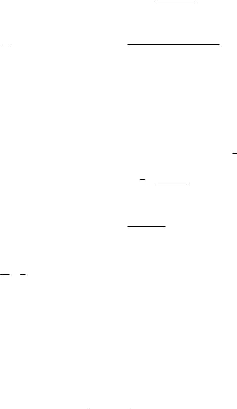
If C(x, 0) is known for t = 0, it is possible to use the result of Sec. 4.8 to determine C(x, t) at any later time. The key to doing this is that if C(x, t) dx is the number of particles in the region between x and x + dx at time t, it may be be interpreted as the probability of finding a particle in the interval (x, dx) multiplied by the total number of particles. (Recall the discussion on p. 91 about the interpretation of C(x, t).) The spreading Gaussian then represents the spread of probability that a particle is between x and x + dx.
If a particle is definitely at x = ξ at t = 0, then σ2(0) = 0. The particle cannot remain there because of equipartition of energy: collisions cause it to acquire a mean square velocity 3kB T /m and move. At some later time
σ(t) = (2Dt)1/2. |
(4.71) |
Define P (ξ, 0; x, t) dx to be the probability that a particle has di used to a location between x and x + dx at time t, if it was at x = ξ when t = 0. This probability is given by Eq. 4.25, except that the distance it has di used is now x − ξ instead of x. The variance σ2(t) is given by Eq. 4.71. The result is
P (ξ, 0; x, t) dx = |
1 |
2 |
|
(4.72) |
||
|
|
|
e−(x−ξ) |
/4Dt dx. |
||
|
|
|||||
√4πDt |
|
|||||
|
|
|
|
|
||
The number of particles initially between x = ξ and x = ξ+dξ is the concentration per unit length times the length of the interval N = C(ξ, 0)dξ, as shown in Fig. 4.19.
The particles can di use in either direction. At a later time t, the average number between x and x + dx that came originally from between x = ξ and x = ξ + dξ is the original number in (ξ, dξ) times the probability that each one got from there to x. This number is a di erential of a di erential, d [C(x, t)dx], because it is only that portion of the particles in dx that came from the interval dξ:
d [C(x, t) dx] = C(ξ, 0) dξ |
1 |
2 |
|
||
|
|
|
e−(x−ξ) |
/4Dt dx. |
|
|
|
||||
√4πDt |
|
||||
|
|
|
|
||
To get C(x, t)dx, it is necessary to integrate over all possible values of ξ:
C(x, t) dx = |
1 |
|
∞ C(ξ, 0)e−(x−ξ)2/4Dt dξ dx. |
|
|
|
|||
√4πDt |
|
|||
|
|
−∞ |
||
|
|
|
|
|
(4.73)
100 4. Transport in an Infinite Medium
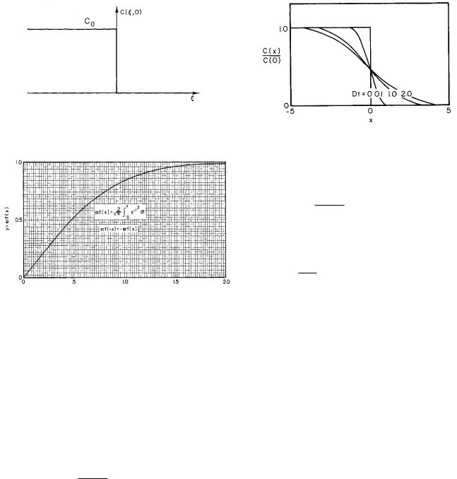
FIGURE 4.20. The initial concentration is constant to the left of the origin and zero to the right of the origin.
FIGURE 4.21. Plot of the error function erf(x).
This equation can be used to find C(x, t) at any time, provided that C(x, t) was known at some earlier time. The factor that multiplies C(ξ, 0) in the integrand is called the influence function or Green’s function for the di u- sion problem; it gives the relative weighting of C(ξ, 0) in contributing to the later value C(x, t).
As an example of using this integral, consider a situation in which the initial concentration has a constant value C0 from ξ = −∞ to ξ = 0 and zero for all positive ξ, as shown in Fig. 4.20. At t = 0 the di usion starts. The concentration at later times is given by
C(x, t) = |
√ |
C0 |
0 |
e−(x−ξ)2/4Dt dξ. |
|
|
|
|
|
|
4πDt |
−∞ |
|
|
|
|
|
Such integrals are most easily evaluated by using the error function that is tabulated in many mathematical tables. It is defined by
√π |
0 |
|
|
||
erf(z) = |
2 |
|
z e−t2 dt. |
(4.74) |
|
|
|
||||
|
|
|
|||
The error function is plotted in Fig. 4.21. One must be careful in using tables, for other functions tabulated are related to the error function but di er in normalization constants and in the limits of integration.
To use the error function in evaluating the integral in Eq. 4.73, make the substitution s = (x − ξ)/(4Dt)1/2.
FIGURE 4.22. The spread of an initially sharp boundary due to di usion.
The integral becomes
|
|
|
|
|
|
|
|
|
|
√ |
|
|
|
|
|
|
|
|
|
|
|
|
C(x, t) = |
|
−C0 |
x/ |
4Dt e−s2 √ |
|
ds. |
|
|||||||||||||
|
|
4Dt |
|
||||||||||||||||||
|
|
|
|
|
√ |
|
|
∞ |
|
|
|
|
|
|
|
|
|
|
|
||
|
|
|
|
|
|
4πDt |
|
|
|
|
|
|
|
|
|
|
|
|
|||
Since |
AB f (x) dx |
= |
0B f (x) dx |
+ |
A0 f (x) dx = |
||||||||||||||||
0B f (x) dx − 0A f (x) dx, this can be written as |
|
||||||||||||||||||||
|
|
|
|
|
x/√ |
|
|
|
|
|
|
∞ |
|
! |
|||||||
|
|
C0 |
|
4Dt |
|
|
s2 |
s2 |
|||||||||||||
C(x, t) = |
− |
|
|
|
|
|
|
e− |
|
ds |
|
|
e− |
ds |
|||||||
√π |
|
|
|
− |
|
||||||||||||||||
|
|
|
0 |
|
|
|
|
|
|
|
|
0 |
|
|
|
||||||
|
= |
C0 |
|
|
|
√ |
|
|
|
|
|
|
|
|
|
|
|||||
|
|
|
|
|
|
|
|
|
|
|
|
|
|||||||||
|
|
|
|
|
1 − erf(x/ |
4Dt) . |
|
|
|
|
|
(4.75) |
|||||||||
|
2 |
|
|
|
|
|
|
|
|
||||||||||||
The plot in Fig. 4.22 shows how the initially sharp concentration step becomes more di use with passing time. Quantitative measurements of the concentration can be used to determine D. Benedek and Villars (2000, pp. 126– 136) discuss some experiments to verify the solution we have obtained above and to determine D.
Many other solutions to the di usion equation and techniques for solving it are known. See Crank (1975) or Carslaw and Jaeger (1959).
4.14 Di usion as a Random Walk
The spreading solution to the one-dimensional di usion equation that we verified can also be obtained by treating the motion of a molecule as a series of independent steps either to the right or to the left along the x axis. (The same treatment can be extended to three dimensions, but we will not do so.) The derivation gives us a somewhat simplified molecular picture of di usion. The derivation also provides an opportunity to see how the Gaussian distribution approximates the binomial distribution. This section is not necessary to understand the rest of Chapters 4 and 5, and you should tackle it only if you are familiar with the binomial and Gaussian probability distributions (Appendices H and I). The model is more restrictive than the di usion equation derived above, since the latter is the linear approximation to the transport problem.

4.14 Di usion as a Random Walk |
101 |
We use a simplified model in which the di using particle always moves in steps of length λ (the mean free path), either in the +x or −x direction. Let the total number of steps taken by the particle be N , of which n are to the right and n are to the left: N = n + n . Also let m = n −n . The particle’s net displacement in the +x direction is then
nλ − n λ = mλ.
Since the steps are independent and a step to the left or right is equally likely (p = 1/2), the probability of having a displacement mλ is given by the binomial probability P (n; N ):
P (n; N ) = |
N ! |
1 n 1 |
n |
(4.76) |
|||
|
|
|
|
|
. |
||
(n!)(N − n)! |
2 |
2 |
|||||
Since this problem is analogous to throwing a coin, and we know that on the average we get the same number of heads (steps to the left) as tails (steps to the right), we know that the distribution is centered at n = n or m = 0. We also know [Eq. G.4] that the variance in n is
given by n2 −n2 = N pq = N/4. Since n = N/2, this says
that n2 = N/4 + N 2/4. However, we need the variance
in m, m2 − m2. To obtain it, we write m = 2n − N and m2 = 4n2 + N 2 − 4nN . Therefore,
m2 = 4n2 + N 2 − 4N n = N.
The variance of the distribution of displacement x is equal to the step length λ times the variance in the number of steps:
σ2 = x2 = λ2m2 = λ2N.
The number of steps is the elapsed time divided by the collision time N = t/tc. Therefore,
σ2 = λ2t . tc
Comparing this with Eq. 4.70, we identify D = λ2/2tc, so that
σ2 = 2Dt. |
(4.77) |
We have shown that this simple model gives a distribution with fixed mean which spreads with a variance proportional to t. We now must show that the shape is Gaussian. Appendix I shows that the Gaussian is an approximation to the binomial distribution in the limit of large N . Since σn2 = N/4 and n = N/2, Eq. G.4 can be used to write
P (n) = 2πN −1/2 e−(n−N/2)2/(2N/4).
4
This can be rewritten in terms of the net number of steps to the right, since m = n − n = 2n − N :
P (m) = |
|
2 |
1/2 e−m2/2N . |
|
πN |
||
|
|
|
FIGURE 4.23. Relationship between the values of x and the allowed values of m. Every other value of m is missing.
Note that only every other value of m is allowed. Since m = 2n − N , m goes in steps of 2 from −N to N as n goes from 0 to N .
To write the probability distribution in terms of x and t, refer to Fig. 4.23. The spacing between each allowed value of x is 2, so that the number of allowed values of m in interval (x, x + dx) is dx/2λ. Therefore, P (x) dx =
P (m)(dx/2λ), |
|
|
|
|
|
|
|
|
|
|
|
P (x) = " |
|
2 |
e−m2/2N . |
||
πN 4λ2 |
|||||
|
|
|
|||
With the substitutions m = x/λ and N = t/tc, this becomes
P (x, t) = |
" |
|
tc |
|
|
e−x2(tc /2λ2t). |
|
|
|
|
|
||
|
|
|
2πλ2t |
|||
With the substitutions D |
= λ2/2tc and C(x, t) = |
|||||
C(0)P (x, t), we obtain Eq. 4.25.
The result of Eq. 4.71 is easily extended to two dimensions. Imagine that a total of N steps are taken, half in the x direction and half in the y direction. Then σx2 = σy2 = λ2(N/2). If r2 = x2 +y2, σr2 = σx2 +σy2 = λ2N . We still define D in any direction as λ2/2tc, where tc is the time between steps in that direction. After a total time t, N steps have been taken, but only half of them were in, say, the x direction. Therefore tc = 2t/N . There-
fore |
|
|
|
|
|
|
σ2 |
= σ2 |
+ σ2 |
= 4Dt (two dimensions). |
(4.78) |
|
r |
x |
y |
|
|
A similar argument in three dimensions gives |
|
||||
σ2 |
= σ2 + σ2 + σ2 = 6Dt (three dimensions). |
(4.79) |
|||
r |
|
x |
y |
z |
|
Figure 4.24 shows the result of a computer simulation of a two-dimensional random walk. A random number is selected to determine whether to step one pixel to the left, up, right, or down—each with the same probability. The trail for 4000 steps is shown in Fig. 4.24(a). The results of continuing for 40,000 steps are shown in Fig. 4.24(b). Note how the particle wanders around one region of space and then takes a number of steps in the same direction to move someplace else. The particle trajectory is “thready.” It does not cover space uniformly. A uniform coverage would be very nonrandom. It is only when many particles are considered that a Gaussian distribution of particle concentration results.
102 4. Transport in an Infinite Medium
(a) |
(b) |
FIGURE 4.24. (a) Trail of a particle for 4000 steps. (b) Trail for additional steps to total 40,000.
Both results in Fig. 4.24 were for the same sequence of random numbers. A computer simulation with 328 runs of 10,000 steps each gave x = −3.3, σx2 = 5142, y = 8.2, σy2 = 4773, and x2 + y2 = 10, 027. The expected values are, respectively, 0, 5000, 0, 5000, and 10,000.
Symbols Used in Chapter 4
Symbol |
Use |
Units |
First |
|
|
|
used on |
|
|
|
page |
a, a1, a2 |
Particle radius |
m |
86 |
b1, b2, b3 |
Constants |
|
93 |
f |
Fraction of cell surface area |
m s−2 |
95 |
g |
Gravitational acceleration |
85 |
|
g |
Force |
N |
87 |
i |
Particle current |
s−1 |
81 |
j, j, js |
Solute fluence rate |
m−2 s−1 |
81 |
jdrift, |
Solute fluence rate due to drift |
m−2 s−1 |
89 |
jdiff |
velocity, di usion |
kg m−2 s−1 |
|
jm |
Mass fluence rate |
81 |
|
jn |
Component of j normal to a sur- |
m−2 s−1 |
83 |
|
face |
m s−1 |
|
jv |
Volume fluence rate |
81 |
|
jx , jy , jz |
Components of j |
m−2 s−1 |
83 |
kB |
Boltzmann’s constant |
J K−1 |
85 |
l |
Linear separation of pores on |
m |
106 |
|
cell surface |
|
|
m |
Mass |
kg |
85 |
m |
n − n |
|
101 |
nˆ |
Unit vector normal to a surface |
|
83 |
n, n |
Number of steps to right, left |
|
101 |
p, q |
Probabilities |
|
101 |
r |
Distance, radius |
m |
83 |
s |
Dummy variable |
|
86 |
t |
Time |
s |
81 |
tc |
Collision time |
s |
86 |
u |
Energy of a particle |
J |
85 |
v, v |
Velocity |
m s−1 |
85 |
x, y, z |
Cartesian coordinates |
m |
81 |
A |
Constant |
|
98 |
B, B |
Cell radius |
m |
95 |
C, Cs |
Concentration |
m−3 |
81 |
D |
Di usion constant |
m2 s−1 |
88 |
F, F, Fext |
Force |
N |
87 |
G |
Correction factor for average |
|
98 |
|
concentration |
|
|
L |
Length |
m |
93 |
M |
Mass |
kg |
84 |
M |
Molecular weight |
|
90 |
N, N0 |
Number of molecules |
|
82 |
N |
Number of pores on cell surface |
|
95 |
N |
Number of steps in a random |
|
101 |
|
walk |
|
|
P |
Rate of energy production |
W |
83 |
|
(power) |
|
|
P |
Probability |
m−3 s−1 |
85 |
Q |
Rate of creating a substance per |
85 |
|
|
unit volume |
J K−1 |
|
R |
Gas constant |
98 |
|
|
|
mol−1 |
|
R |
Radius of a sphere |
m |
94 |
Rp |
Radius of a pore |
m |
94 |
S |
Surface area |
m2 |
82 |
dS |
Vector surface element pointing |
m2 |
83 |
|
in the direction of the normal |
|
|
T |
Absolute temperature |
K |
85 |
V |
Volume |
m3 |
84 |
∆Z |
Cell membrane thickness |
m |
94 |
α |
Proportionality constant |
N s m−1 |
87 |
β |
Proportionality constant |
87 |
|
|
between force and velocity |
J K−1 m−1 |
|
κ |
Thermal conductivity |
88 |
|
|
|
s−1 |
|
λ |
Mean free path |
m |
86 |
λ |
Ratio of D/v |
m |
98 |
θ, φ |
Angles |
|
82 |
η |
Coe cient of viscosity |
Pa s |
88 |
σ |
Standard deviation |
Ω−1 m−1 |
91 |
σ |
Electrical conductivity |
88 |
|
ξ |
Position |
m |
99 |
ξ |
Dimensionless variable |
kg m−3 |
98 |
ρ |
Mass density |
84 |
|
µs |
Chemical potential of solute |
J |
88 |
|
|
molecule−1 |
|
Problems
Section 4.1
Problem 1 A cylindrical pipe with a cross-sectional area S = 1 cm2 and length 0.1 cm has js(0)S = 200 s−1 and js(0.1)S = 150 s−1.
(a)What is the total rate of buildup of particles in the
pipe?
(b)What is the average rate of change of concentration in the section of pipe?
Problem 2 Write the continuity equation in cylindrical coordinates if jφ = 0 but jr and jz can be nonzero.
Problem 3 Consider two concentric spheres of radii r and r + dr. If the particle fluence rate points radially and depends only on r, and the number of particles between r and r + dr is not changing, show that d(r2j)/dr = 0.
Section 4.2
Problem 4 Suppose that the total blood flow through a region is F (m3 s−1). A chemically inert substance is carried into the region in the blood. The total number of molecules of the substance in the region is N . The amount of blood in the region is not changing. Show that dN/dt = (CA −CV )F , where CA and CV are the concentrations of substance in the arterial and venous blood. This is known

as the Fick principle or the Fick tracer method. It is often used with radioactive tracers.
Section 4.3
Problem 5 R. D. Allen et al. [(1982). Science 218: 1127–1129] report seeing regular movement of particles in the axoplasm of a squid axon. At a temperature of 21 ◦C, the following mean drift speeds were observed:
Particle size (µm) Typical speed (µm s−1)
0.8 − 5.0 |
0.8 |
0.2 − 0.6 |
2 |
How do these values compare to thermal speeds? (Make a reasonable assumption about the density of particles and assume that they are spherical.)
Section 4.4
Problem 6 (a) Use the ideal gas law, pV = N kB T = nRT to compute the volume of 1 mole of gas at T = 30 ◦C and p = 1 atm . Express your answer in liters. Show that
this is equivalent to a concentration of 2.4×1025 molecule m−3.
(b) Find the concentration of liquid water molecules at room temperature.
Problem 7 Using the information on the mean free path in the atmosphere and assuming that all molecules have a molecular weight of 30, find the height at which the mean free path is 1 cm. Assume the atmosphere has a constant temperature.
Section 4.6
Problem 8 Suppose C(x, t) = N/√4πDt e−x2/4Dt.
Find an expression for js(x, t).
Section 4.7
Problem 9 If all macromolecules have the same density, derive the expression for D versus the molecular weight that was used to draw the line in Fig. 4.12.
Problem 10 For diagnostic studies of the lung, it would be convenient to have radioactive particles that tag the air and that are small enough to penetrate all the way to the alveoli. It is possible to make the isotope 99mTc into a “pseudogas” by burning a flammable aerosol containing it. The resulting particles have a radius of about 60 nm [W. M. Burch, I. J. Tetley, and J. L. Gras (1984). Clin. Phys. Physiol. Meas 5: 79–85]. Estimate the mean free path for these particles. If it is small compared to the molecular diameter, then Stokes’ law applies, and you can use Eq. 4.23 to obtain the di usion constant. (The viscosity of air at body temperature is about 1.8×10⁻⁵ Pa s.)
Problems 103
Problem 11 Figure 4.12 shows that D for O2 in water at 298 K is 1.2 × 10⁻⁹ m2 s−1 and that the molecular radius of O2 is 0.2 nm. The di usion constant of a dilute gas (where the mean free path is larger than the molecular diameter) is D = λ2/2tc, where the collision time is given by Eq. 4.15.
(a)Find a numeric value for the di usion constant for O2 in O2 at 1 atm and 298 K and its ratio to D for O2 in water. The molecular weight of oxygen is 32.
(b)Assuming that this equation for a dilute gas is valid in water, estimate the mean free path of an oxygen molecule in water.
Section 4.8
Problem 12 (a) The three-dimensional normalized analog of Eq. 4.25 is
C(x, y, z, t) = |
N |
exp |
|
x2 + y2 + z2 |
|
|
|
− |
|
|
. |
||
[2π σ2(t)]3/2 |
2σ2(t) |
|||||
Find the three-dimensional analog of Eq. 4.27.
(b) Show that σ2 = x2 + y2 + z2 = 6Dt.
Problem 13 A crude approximation to the Gaussian probability distribution is a rectangle of height P0 and width 2L. It gives a constant probability for a distance L either side of the mean.
(a)Determine the value of P0 and L so that the distribution has the same value of σ as a Gaussian.
(b)Plot P (x, t) if σ is given by Eq. 4.27 and the mean remains centered at the origin for times of 1, 5, 50, 100, and 500 ms. Use D for oxygen di using in water at body temperature.
(c)How long does it take for the oxygen to have a reasonable probability of di using a distance of 8 µm, the diameter of a capillary?
(d)For t = 100 ms, plot both the accurate Gaussian and the rectangular approximation.
Problem 14 Write an equation for Fick’s second law in three-dimensional Cartesian coordinates when the di u- sion constant depends on position: D = D(x, y, z).
Problem 15 The heat flow equation in one dimension is
|
∂T |
|
jH = −κ |
|
, |
∂x |
where κ is the thermal conductivity in W m−1 K−1. One often finds an equation for the “di usion” of energy by heat flow:
∂T |
= DH |
|
∂2T |
. |
∂t |
|
|||
|
|
∂x2 |
||
The units of jH are J m−2 s−1. The internal energy per unit volume is given by u = ρCT , where C is the heat capacity per unit mass and ρ is the density of the material. Derive the second equation from the first and show how DH depends on κ, C, and ρ.

104 4. Transport in an Infinite Medium
Problem 16 The dimensionless “Lewis number” is defined as the ratio of the di usion constant for molecules and the di usion constant for heat flow (see Problem 15.) If the Lewis number is large, molecular di usion occurs much more rapidly than the di usion of energy by heat flow. If the Lewis number is small, energy di uses more rapidly than molecules. Use the following parameters:
|
Air |
Water |
D (m2 s−1) |
2 × 10⁻⁵ |
2 × 10⁻⁹ |
κ (W m−1 K−1) |
0.03 |
0.6 |
C (J kg−1 K−1) |
1000 |
4000 |
ρ (kg m−3) |
1.2 |
1000. |
(a)Calculate the Lewis number for oxygen in air and in water.
(b)Is it possible using either air or water to design a system in which oxygen is transported by di usion with almost no transfer of heat?
Problem 17 A sheet of labeled water molecules starts at the origin in a one-dimensional problem and di uses in the x direction.
(a)Plot σ vs t for di usion of water in water.
(b)Deduce a “velocity” versus time.
(c)How long does it take for the water to have a reasonable chance of traveling 1 µm? 10 µm? 100 µm? 1 mm? 1 cm? 10 cm?
Problem 18 In three dimensions the root-mean-square
√
di usion distance is σ = 6Dt, where t is the di usion time. Consider the di usion of oxygen from air to the blood in the lungs. The terminal air sacs in the lungs, the alveoli, have a radius of about 100 µm. The radius of a capillary is about 4 µm. Estimate the time for an oxygen molecule to di use from the center to the edge of an alveolus, and the time to di use from the edge to the center of a capillary. Which is greater? From the data in Table 1.4 estimate how long blood remains in a capillary. Is it long enough for di usion of oxygen to occur? Assume the di usion constant of oxygen in air is 2 ×10⁻⁵ m2 s−1 and in water is 2 × 10⁻⁹ m2 s−1.
Problem 19 Why breathe? Estimate the time required for oxygen to di use from our nose to our lungs. Assume the di usion constant of oxygen in air is 2×10⁻⁵ m2 s−1.
Problem 20 At a nerve-muscle junction, the signal from the nerve is transmitted to the muscle by a chemical junction or synapse. In order to activate a muscle, molecules of acetylcholine (ACh) must di use from the end of the nerve cell across an extracellular gap about 20 nm wide to the muscle cell. Assuming one-dimensional di u- sion, estimate the signal delay caused by the time needed for ACh to di use. The delay of the signal at the nervemuscle junction is about 0.5 ms. How does this compare to
the di usion time? Use a di usion constant of 5 × 10⁻¹⁰ m2 s−1.
Problem 21 A substance has di usion constant D, and
its concentration is distributed in |
space according to |
C(x, t) = A(t) sin(2πx/L), where |
L is the wavelength |
and A(t) is the amplitude of the distribution. Use the one-dimensional di usion equation, Eq. 4.26, to show that the concentration decays exponentially with time, A(t) e−t/τ . Determine an expression for the time constant τ in terms of L and D. Which decays faster: a longwavelength (di use) distribution, or a short-wavelength (localized) distribution? This result can be used with the Fourier methods developed in Chapter 11 to derive very general solutions to the di usion equation.
Problem 22 Some tissues, such as skeletal muscle, are anisotropic: the rate of di usion depends on direction. In these tissues, Fick’s first law in two dimensions has the form
jx |
Dxx |
Dxy |
∂C/∂x |
jy |
= − Dyx |
Dyy |
∂C/∂y . |
The 2 × 2 matrix is called the “di usion tensor.” It is always symmetric, so Dxy = Dyx.
(a) Derive the two-dimensional di usion equation for anisotropic tissue. Assume the di usion tensor depends on direction but not on position.
(b) If the coordinate system is rotated from (x, y) to
(x , y ) by |
|
|
|
|
|
|
|
|
x |
= |
cos θ |
sin θ |
x |
, |
|
|
y |
− |
sin θ |
cos θ |
y |
||
|
|
|
|||||
|
|
|
|
|
|
|
|
the di usion tensor changes by |
|
|
|||||
Dx x Dx y |
|
|
|
|
|
|
|
Dx y Dy y |
|
|
|
|
|
|
|
= cos θ |
sin θ Dxx |
Dxy cos θ |
− sin θ . |
||||
− sin θ |
cos θ |
Dxy |
Dyy |
sin θ |
cos θ |
||
Find the angle θ such that the tensor is diagonal (Dx y = 0). Typically, this direction is parallel to a special direction in the tissue, such as the direction of fibers in a muscle.
(c) Show that the trace of the di usion tensor (the sum of the diagonal terms) is the same in any coordinate system (Dxx + Dyy = Dx x + Dy y for any θ). Basser et al. (1994) invented a way to measure the di usion tensor using magnetic resonance imaging (Chapter 18). From the di usion tensor they can image the direction of the fiber tracts. When they want images that are independent of the fiber direction, they use the trace.
Problem 23 Calcium ions di use inside cells. Their concentration is also controlled by a bu er:
Ca + B CaB.
The concentrations of free calcium, unbound bu er, and bound bu er ([Ca], [B], and [CaB]) are governed, assum-