Intermediate Physics for Medicine and Biology - Russell K. Hobbie & Bradley J. Roth

64 3. Systems of Many Particles

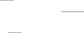
FIGURE 3.13. Two systems that can exchange volume are separated by a movable piston. Heat can also flow through the piston.

V = V + V and U = U + U from which dV = −dV , dU = −dU . As before, equilibrium exists when the total number of microstates or the total entropy is a maximum. The conditions for maximum entropy are

The derivation proceeds as before. For example,

Equilibrium requires that T = T so that there is no heat flow. The piston will stop moving and there will be no change of volume when

These derivatives can be evaluated in several ways. The method used here involves some manipulation of derivatives; a more detailed description, consistent with the microscopic picture of energy levels, is found in Reif (1964, pp. 267–273).

For a small exchange of heat and work, the first law can be written as dU = dQ−dW . In the present case the only form of work is that related to the change of volume, so dU = dQ−pdV . It was shown in Eq. 3.23 that dQ = T dS. Therefore dU = T dS −pdV . This equation can be solved for dS:

The entropy depends on U ,V and N : S = S(U, V, N ).

Comparison of this with Eq. 3.52 shows that

The first of these equations was already seen as Eq. 3.21. The second gives the condition for equilibrium under volume change. Referring to Eq. 3.51 we see that at equilibrium

This agrees with common experience. The piston does not move when the pressure on each side is the same.

3.15Extensive Variables and Generalized Forces

The number of microstates and the entropy of a system depend on the number of particles, the total energy, and the positions of the energy levels of the system. The positions of the energy levels depend on the volume and may also depend on other macroscopic parameters. For example, they may depend on the length of a stretched muscle fiber or a protein molecule. For charged particles in an electric field, they depend on the charge. For a thin film such as the fluid lining the alveoli of the lungs, the entropy depends on the surface area of the film. The number of particles, energy, volume, electric charge, surface area, and length are all extensive variables: if a homogeneous system is divided into two parts, the value of the variable for the total system (volume, charge, etc.) is the sum of the values for each part. A general extensive variable will be called x.

An adiabatic energy change is one in which no heat flows to or from the system. The energy change is due to work done on or by the system as a macroscopic parameter changes, shifting at least some of the energy levels. For each extensive variable x we can define a generalized force X such that the energy change in an adiabatic process is

(Remember that dU is the increase in energy of the system and dW is the work done by the system on the surroundings.) Examples of extensive variables and their associated forces are given in Table 3.4.

3.16The General Thermodynamic Relationship

Suppose that a system has N particles, total energy U , volume V , and another macroscopic parameter x on which the positions of the energy levels may depend. The

TABLE 3.4. Examples of extensive variables and the generalized force associated with them.

number of microstates, and therefore the entropy, will depend on these four variables: S = S(U, N, V, x). If each variable is changed by a small amount, there is a change of entropy

Now consider the change of energy of the system. If only heat flow takes place, there is an increase of energy dQ = T dS. If an adiabatic process with a constant number of particles takes place, the energy change is −dW = Xdx − pdV . If particles flow into the system without an accompanying flow of heat or work, the energy change is dUN . It seems reasonable that this energy change, due solely to the movement of the particles, is proportional to dN : dUN = a dN . (It will turn out that the proportionality constant is the chemical potential.) For the total change of energy resulting from all these processes, we can write a statement of the conservation of energy: dU = T dS + Xdx − pdV + adN . This is an extension of Eq. 3.5 to the additional variables on which the energy can depend. It can be rearranged as

Comparison of Eqs. 3.57 and 3.58 shows that

Comparison of Eq. 3.59b with Eq. 3.45 shows that a = µ. This is why the factor of T was introduced in Eq. 3.45.

Equation 3.58, with the correct value inserted for a, is

between entropy change and heat flow in a reversible process. (A reversible process is one that takes place so slowly that all parts of the system have the same temperature, pressure, etc.) This equation and derivative relations such as Eqs. 3.59 form the basis for the usual approach to thermodynamics.

Finally, let us consider the addition of a particle to a system when the volume is fixed. If we do this without changing the energy, it increases the number of ways the existing energy can be shared and hence the number of microstates. Therefore the entropy increases. If we want to restore the entropy to its original value, we must remove some energy. Exactly the same argument can be made mathematically. We have seen in Eqs. 3.45 and 3.59b that

Since adding the particle at constant energy increases the entropy, (∂S/∂N )U,V is positive and the chemical potential is negative. Next, we rearrange Eq. 3.60 as dU = T dS + µ dN − p dV and by inspection see that

Therefore adding a particle at constant volume while keeping the entropy constant requires that energy be removed from the system.

3.17 The Gibbs Free Energy

3.17.1Gibbs Free Energy

A conventional course in thermodynamics develops several functions of the entropy, energy, and macroscopic parameters that are useful in certain special cases. One of these is the Gibbs free energy, which is particularly useful in describing changes that occur in a system while the temperature and pressure remain constant. Most changes in a biological system occur under such conditions.

Imagine a system A in contact with a much larger reservoir as in Fig. 3.14. The reservoir has temperature T and

A'

AV V' U U'

This is known as the thermodynamic identity or the fundamental equation of thermodynamics. It is a combination of the conservation of energy with the relationship

FIGURE 3.14. System A is in contact with reservoir A . Heat can flow through the piston, which is also free to move. The reservoir is large enough to ensure that anything that happens to system A takes place at constant temperature and pressure.

66 3. Systems of Many Particles

pressure p . A movable piston separates A and A . (At equilibrium, T = T and p = p .) The reservoir is large enough so that a change of energy or volume of system A does not change T or p .

Consider the change of entropy of the total system that accompanies an exchange of energy or volume between A and A . Above, this entropy change was set equal to zero to obtain the condition for equilibrium. In this case, however, we will express the total entropy change of system plus reservoir in terms of the changes in system A alone. The total entropy is S = S + S , so the total entropy change is dS = dS + dS .

If reservoir A exchanges energy with system A, the energy change is

dU = T dS − dW = T dS − p dV .

This can be solved for dS , and the result can be put in the expression for the total entropy change:

We are trying to get dS in terms of changes in system A alone. Since A and A together constitute an isolated system, dU = −dU and dV = −dV . Therefore,

(Note that a minus sign was introduced in front of this equation.) This expresses the total entropy change in terms of changes of S, U , and V in system A and the pressure and temperature of the reservoir.

The Gibbs free energy is defined to be

If the reservoir is large enough so that interaction of the system and reservoir does not change T and p , then the change of G as system A changes is

The change in entropy of system plus reservoir is related to the change of G, which is a property of the system alone, as long as the pressure and temperature are maintained constant by the reservoir.

To see why G is called a free energy, consider the conservation of energy in the following form:

(work done by the system) = (energy lost by the system)

+ (heat added to the system),

dW = −dU + T dS.

Subtracting pdV from both sides of this equation gives

dW − p dV = −dU + T dS − p dV = −dG.

The right-hand side is the decrease of Gibbs free energy of the system. The work done in any isothermal, isobaric (constant pressure) reversible process, exclusive of pdV work, is equal to the decrease of Gibbs free energy of the system. This non–p dV work is sometimes called useful work. It may represent contraction of a muscle fiber, the transfer of particles from one region to another, the movement of charged particles in an electric field, or a change of concentration of particles. It di ers from the change in energy of the system, dU , for two reasons. The volume of the system can change, resulting in p dV work, and there can be heat flow during the process. For example, let the system be a battery at constant temperature and pressure which decreases its internal (chemical) energy and supplies electrical energy. From a chemical energy change dU we subtract T dS, the heat flow to the surroundings, and −p dV , the work done on the atmosphere as the liquid in the battery changes volume. What is left is the energy available for electrical work.

3.17.2An Example: Chemical Reactions

As an example of how the Gibbs free energy is used, consider a chemical reaction that takes place in the body at constant temperature and pressure. System A, the region in the body where the reaction takes place, is in contact with a reservoir A that is large enough to maintain constant temperature and pressure. Suppose that there are four species of particles that interact. Capital letters represent the species and small letters represent the number of atoms or molecules of each that enter in the reaction:

aA + bB ←→ cC + dD.

An example is 1 glucose+6O2 ←→6CO2+6H2O, where a = 1, b = 6, c = 6, d = 6. The state of the system depends on U , V , NA, NB , NC , and ND .

We begin with the definition of G, Eq. 3.62, and we call the pressure and temperature of the system and reservoir p and T :

G = U − T S + pV.

Di erentiating, we obtain

dG = dU − T dS − S dT + p dV + V dp.

Generalize Eq. 3.60 for the case of four chemical species:

T dS = dU −µA dNA −µB dNB −µC dNC −µD dND +p dV.

Insert this in the equation for dG and remember that since the process takes place at constant temperature and pressure, dT and dp are both zero. The result is

dG = µA dNA + µB dNB + µC dNC + µD dND .

In Sec. 3.13 we saw that the concentration dependence of the chemical potential is given by a logarithmic term. Equation 3.48 can be used to write

µA = µA0 + kB T ln(CA/C0),

where µA0 is the chemical potential at a standard concentration (usually 1 mol) and depends on temperature, pH, etc. Note that C0 is the same reference concentration for all species. As the reaction takes place to the right, we can write the number of molecules gained or lost as

The two logarithm terms together represent logs of concentration ratios. Therefore concentrations [A], [B], [C], [D], and C0 must all be measured in the same units. The last term can be made to vanish if the units are such that C0 is unity (for example, 1 mol per liter). Then

dG = [cµC0 + dµD0 − aµA0 − bµB0

Multiplying the expression in square brackets by Avogadro’s number converts the chemical potential per molecule to the standard Gibbs free energy per mole, and kB T to RT . To compensate, the change in number of molecules dN is changed to moles dn or ∆n:

The term in small parentheses is the standard free energy change for this reaction, ∆G0, which can be found in tables. At equilibrium ∆G = 0, so

0 = ∆G0 + RT ln [C]c[D]d = ∆G0 + RT ln Keq. [A]a[B]b

The equilibrium constant Keq is related to the standard (1 molar) free-energy change by

∆G0 = −RT ln Keq,

Keq = [A]a[B]b .

Many biochemical processes in the body receive free energy from the change of adenosine triphosphate (ATP) to adenosine diphosphate (ADP) plus inorganic phosphate (Pi). This reaction involves a decrease of free energy. The energy is provided initially by forcing the reaction to go in the other direction to make an excess of ATP. One way this is done is through a very complicated series of chemical reactions known as the respiration of glucose. The net e ect of these reactions is11

The decrease in free energy of the glucose more than compensates for the increase in free energy of the ATP. The creation of glucose or other sugars is the reverse of the respiration process and is called photosynthesis. The free energy required to run the reaction the other direction is supplied by light energy.

3.18The Chemical Potential of a Solution

We now consider a binary solution of solute and solvent and how the chemical potential changes as these two substances are intermixed.12 This is a very fundamental process that will lead us to the logarithmic dependence of the chemical potential on solute concentration that we saw in Sec. 3.13, as well as to an expression for the chemical potential of the solvent that we will need in Chapter 5.

To avoid having the subscript s stand for both solute and solvent, we call the solvent water. The distinction between solute and water is artificial; the distinction is usually that the concentration of solute is quite small. We need the entropy change in a solution when Ns solute molecules, which initially were segregated, are mixed with Nw water molecules. We make the calculation for an ideal solution—one in which the total volume of water molecules does not change on mixing and in which there is no heat evolved or absorbed on mixing. This is equivalent to saying that the solute and water molecules are the same size and shape, and that the force between a water molecule and its neighbors is the same as the force between a solute molecule and its neighbors.13 The resulting entropy change is called the entropy of mixing.

To calculate the entropy of mixing, imagine a system with N sites, all occupied by particles. The number of microstates is the number of di erent ways that particles can be placed in the sites. The first particle can go in any

11There are multiple pathways in glucose respiration. The 36 is approximate.

12See also Hildebrand and Scott (1964), p. 17, and Chapter 6.

13Extensive work has been done on solutions for which these assumptions are not true. See Hildebrand and Scott (1964); Hildebrand et al. (1970).

68 3. Systems of Many Particles

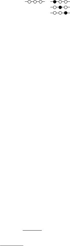
FIGURE 3.15. The system on the left contains three water molecules. Because they are indistinguishable there is only one way they can be arranged. The system on the right contains two water molecules and one solute molecule. Three different arrangements are possible. In each case the number of arrangements in given by (Nw + Ns)!/(Nw !Ns!).

site. The second can go in any of N −1 sites, and so forth. The total number of di erent ways to arrange the particles is N ! But if the particles are identical, these states cannot be distinguished, and there is actually only one microstate. The number of microstates is N !/N !, where the N ! in the numerator gives the number of arrangements and the N ! in the denominator divides by the number of indistinguishable states.14

Suppose now that we have two di erent kinds of particles. The total number is N = Nw + Ns, and the total number of ways to arrange them is (Nw + Ns)! The Nw water molecules are indistinguishable, so this number must be divided by Nw ! Similarly it must be divided by Ns! Therefore, purely because of the ways of arranging the particles, the number of microstates Ω in the mixture is (Nw + Ns)!/ (Nw ! Ns!) . An example of counting microstates is shown in Fig. 3.15.

There could also be dependence on volume and energy; in fact, the dependence on volume and energy may also contain factors of Nw and Ns. However, our assumption that the molecules of water and solute have the same size, shape, and forces of interaction ensures that these dependencies will not change as solute molecules are mixed with water molecules. The only entropy change will be the entropy of mixing.

The entropy change of the mixture relative to the entropy of Nw molecules of pure water and Ns molecules of pure solute is

pure solute

Since with our assumptions Ω is unity for the pure solute and the pure water, the entropy di erence is

Ssolution − Spure water, pure solute

= kB ln

(Nw + Ns)!

Nw ! Ns!

= kB {ln [(Nw + Ns)!] − ln(Nw !) − ln(Ns!)} . (3.67)

14The fact that there is only one microstate because of the indistinguishability of the particles is called the Gibbs paradox. For an illuminating discussion of the Gibbs paradox, see Casper and Freier (1973).

This is symmetric in water and solute, and it is valid for any number of molecules.

Since we usually deal with large numbers of molecules and factorials are di cult to work with, let us use Stirling’s approximation (Appendix I) to write

= kB [(Nw + Ns) ln(Nw + Ns) − Nw ln Nw − Ns ln Ns] .

The next step is to relate the entropy of mixing to the chemical potential. This is done by recalling the definition of the Gibbs free energy, (Eq. 3.62): G = U + p V − T S. The sum of the first two terms, H = U + p V , is called the enthalpy. Any change of the enthalpy is the heat of mixing; in our case it is zero. (The present case is actually more restrictive: p, V , and U are all constant.) Therefore, since T is also constant, the change in Gibbs free energy is due only to the entropy change:

This is still symmetric with water and solute, but it diverges if either Nw or Ns is zero, because of our use of Stirling’s approximation.

We now need an expression that relates the change in G to the chemical potential. This can be derived for the general case using the following thermodynamic arguments. We use Eq. 3.62 to write the most general change in G:

dG = dU + p dV + V dp − T dS − S dT.

The fundamental equation of thermodynamics, Eq. 3.60, generalized to two molecular species, is

T dS = dU − µw dNw − µs dNs + p dV,

so

This can be used to write down some partial derivatives by inspection that are valid in general:

To find the chemical potential, we di erentiate our expression for G, Eq. 3.69, with respect to Nw and Ns to obtain

These have been written in terms of the mole fractions or molecular fractions

Each chemical potential is zero when the mole fraction for that species is one (i.e., the pure substance). The expressions for µ diverge for xw or xs close to zero because of the failure of Stirling’s approximation for small values of x.

The last step is to write the chemical potential in terms of the more familiar concentrations instead of mole fractions. We can write the change in chemical potential of the solute as the concentration changes from a value C1 to C2 as

∆µs = µs(2) − µs(1) = kB T ln(x2/x1).

As long as the solute is dilute, Nw +Ns ≈ Nw , so x2/x1 =

C2/C1 and

∆µs = kB T ln(C2/C1),

which agrees with Eq. 3.48.

The change in chemical potential of the water can be written in terms of the solute concentration. Since xw + xs = 1, µw = kB T ln(1 − xs). For small values of xs the logarithm can be expanded in a Taylor’s series (Appendix

D):

ln(1 − xs) = −xs − 12 x2s − · · · . The final result is

µw = −kB T xs = −kB T Ns/(Ns + Nw ) ≈ −kB T (Ns/V )/(Nw /V ),

or

To reiterate, this is the chemical potential of the water for small solute concentrations. The zero of chemical potential is pure water. The term is negative because the addition of solute decreases the chemical potential of the water, due to the entropy of mixing term. For a change of solute concentration, the chemical potential of the water changes by

We now know the concentration dependence of the chemical potential. In Chapter 5 we will be concerned with the movement of solute and water, and we will need to know the dependence of the chemical potentials on pressure. To find this, we write

The second term is just Eq. 3.74b. To obtain the derivative in the first term, we use the fact that when the

partial derivative of a function is taken with respect to two variables, the result is independent of the order of di erentiation (Appendix N):

For a process at constant temperature, the rate of change of µw with p for constant solute concentration is the same as the rate of change of V with Nw when p is fixed.

The quantity (∂V /∂Nw )T,p is the rate at which the volume changes when more molecules are added at constant temperature and pressure. For an ideal incompressible liquid it is the molecular volume, V w . We can repeat this argument for the solute to obtain

In a solution, the total volume is V = Nw V w + NsV s where V w and V s are the average volumes occupied by one molecule of water and solute. Dividing by V gives 1 = Cw V w + CsV s. If the solution is dilute,

In an ideal solution V w = V s. For an ideal dilute solution, we then have

∆µw = V w (∆p − kB T ∆Cs) ≈ ∆p − kB T ∆Cs . (3.78)

Cw

∆µs = kB T ln(Cs2/Cs1) + V s ∆p

We saw this concentration dependence earlier, in Sec. 3.13. If the concentration di erence is small, we can write Cs2 = Cs1 + ∆Cs and use the expansion ln(1 + x) ≈ x to obtain

3.19Transformation of Randomness to Order

When two systems are in equilibrium, the total entropy is a maximum. Yet a living creature is a low-entropy, highly ordered system. Are these two observations in conflict? The answer is no; the living system is not in equilibrium, and it is this lack of equilibrium that allows the entropy to

70 3. Systems of Many Particles

be low. The conditions under which order can be brought to a system—its entropy can be reduced—are discussed briefly in this section.

A car travels with velocity v and has kinetic energy 12 mv2. In addition to the random thermal motions of the atoms making up the car, all the atoms have velocity v in the same direction (except for those in rotating parts, which have an ordered velocity that is more complicated to describe). If the brake shoes are brought into contact with the brake drums, the car loses kinetic energy, and the shoes and drums become hot. Ordered energy has been converted into disordered, thermal energy; the entropy has increased. Is it possible to heat the drums and shoes with a torch, apply the brakes, and have the car move as the drums and shoes cool o ? Energetically, this is possible, but there are only a few microstates in which all the molecules are moving in a manner that constitutes movement of the car. Their number is vanishingly small compared to the number of microstates in which the brake drums are hot. The probability that the car will begin to move is vanishingly small.

An animal is placed in an insulated, isolated container. The animal soon dies and decomposes. Energetically, the animal could form again, but the number of microstates corresponding to a live animal is extremely small compared to all microstates corresponding to the same total energy for all the atoms in the animal.

In some cases, thermal energy can be converted into work. When gas in a cylinder is heated, it expands against a piston that does work. Energy can be supplied to an organism and it lives. To what extent can these processes, which apparently contradict the normal increase of entropy, be made to take place? These questions can be stated in a more basic form.

1.To what extent is it possible to convert internal energy distributed randomly over many molecules into energy that involves a change of a macroscopic parameter of the system? (How much work can be captured from the gas as it expands the piston?)

2.To what extent is it possible to convert a random mixture of simple molecules into complex and highly organized macromolecules?

Both these questions can be reformulated: under what conditions can the entropy of a system be made to decrease?

The answer is that the entropy of a system can be made to decrease if, and only if, it is in contact with one or more auxiliary systems that experience at least a compensating increase in entropy. Then the total entropy remains the same or increases. This is one form of the second law of thermodynamics. For a fascinating discussion of the second law, see Atkins (1994).

One device that can accomplish this process is a heat engine. It operates between two thermal reservoirs at different temperatures, removing heat from the hotter one

and injecting heat into the cooler one. Even though less heat goes into the cooler reservoir than was removed from the hotter one (the di erence being the mechanical work done by the engine), the overall entropy of the two reservoirs increases. The entropy change of the hot reservoir is a decrease, −∆Q/T , while the entropy change of the cooler reservoir is an increase, +∆Q /T . Since T < T , the entropy increase more than balances the decrease, even though ∆Q < ∆Q. The increase in the number of accessible microstates of the cooler reservoir is greater than the decrease in the number of accessible microstates of the hotter reservoir. The coupled chemical reactions that we saw in Sec. 3.17 are analogous.

Symbols Used in Chapter 3

72 3. Systems of Many Particles

carry an XX chromosome pair, while males have an XY pair. The trait is recessive, which means that the patient exhibits color blindness only if there is no normal X gene present. Let Xd be a defective gene. Then for a female, the possible gene combinations are

XX, XXd, XdXd.

For a male, they are

XY, XdY.

In a large population about 8% of the males are colorblind. What percentage of the females would you expect to be color-blind?

Problem 7 A patient with heart disease will sometimes go into ventricular fibrillation, in which di erent parts of the heart do not beat together, and the heart cannot pump. This is cardiac arrest. The following data show the fraction of patients failing to regain normal heart rhythm after attempts at ventricular defibrillation by electric shock [W. D. Weaver (1982). New Engl. J. Med. 307: 1101– 1106.]

Assume that the probability p of defibrillation on one attempt is independent of other attempts. Obtain an equation for the probability that the patient remains in fibrillation after N attempts. Compare it to the data and estimate p.

Problem 8 There are N people in a class (N = 25). What is the probability that no one in the class has a birthday on a particular day? Ignore seasonal variations in birth rate and ignore leap years.

Problem 9 The death rate for 75-year-old people is 0.089 per year (Commissioners 1941 Standard Ordinary Mortality Table).

(a)What is the probability that an individual aged 75 will die during a 12-hour period? Neglect the fact that some are sick, some are terminally ill, and so on, and assume that the probability is the same for everyone.

(b)Suppose that 10, 000 people, all aged 75, are given the flu vaccine at t = 0. What is the probability that none will die during the next 12 hours? (This underestimates the probability, since sick people would not be given the vaccine, but they are included in the death rate.)

Problem 10 This problem is intended to help you understand some of the nuances of the binomial probability distribution.

(a)In a macabre “game” of “roulette” the victim places one bullet in the cylinder of a revolver. (A less hazardous game could be done with dice.) There is room for six bullets in the cylinder. The victim spins the cylinder, so there is a probability of 1/6 that the bullet is in firing position. The victim then places the gun to the head and fires. If the victim survives, the cylinder is spun again and the process is repeated. We can look either at the cumulative probability of “success” (being killed), or the cumulative probability of “failure” (surviving). Make a table for 1000 victims who keep playing the game over and over. Plot the number surviving, the number killed on each try, and the cumulative number killed.

(b)Show that the number surviving can be expressed as 1000e−bN , where N is the number of tries, and find b.

(c)The data in the following table are from F´ed´eration CECOS, D. Schwartz and M. J. Mayaux (1982). Female fecundity as a function of age, N. Engl. J. Med. 306(7): 404–406. They show the cumulative success rates in different age groups for patients being treated for infertility by artificial insemination from a donor. That is, each month at the time of ovulation each patient who has not yet become pregnant is inseminated artificially. Plot these data. What do they suggest? Make whatever plots can confirm or rule out what you suspect.

Section 3.3

Problem 11 A thermally insulated ideal gas of particles is confined within a container of volume V . The gas is initially at absolute temperature T . The volume of the container is very slowly reduced by moving a piston that constitutes one wall of the container. Give qualitative answers to the following questions.

(a)What happens to the energy levels of each particle?

(b)Is the work done on the gas as its volume decreases positive or negative?

(c)What happens to the energy of the gas?

Section 3.5

Problem 12 System A has 1020 microstates, and system A has 1019 microstates. How many microstates does the combined system have?

Problem 13 Calculate the Celsius and absolute temperatures corresponding to a room temperature of 68 ◦F, a normal body temperature of 98.6 ◦F, and a febrile body temperature of 104 ◦F.

Problem 14 Calculate and plot Ω, Ω , and Ω for Fig. 3.10, thus reproducing the figure. Write down an analytic expression for Ω and di erentiate to find the value of U for which Ω is a maximum.

Problem 15 Systems A and A each consist of three particles, whose energy levels are u, 2u, 3u, etc. The total energy available to the combined system is U = 12u.

(a)Make a table similar to Table 3.3. (If you have di culty, see part (d) of this problem.)

(b)Find the most probable state. To what values of U and U does it correspond?

(c)Plot Ω vs. U. What is the probability that all three particles in system A have energy u?

(d)Consider system A. If it has energy U, the maximum energy the first particle can have is U − 2u. How many microstates are there for which the first particle has energy U − 2u? U − 3u? Show that the total number of microstates for system A is given by

This proves the assertion in the text that for 3 particles, Ω increases as U 2.

Problem 16 We have seen that in general with volume, number of particles, and other parameters that determine the positions of the energy levels held fixed,

Suppose that U = CT , where C is the heat capacity of the system. Find Ω(U ).

Problem 17 Systems A and A are in thermal contact. Show that if T < T , energy flows from A to A to increase Ω , while if T > T , energy flows from A to A .

Problem 18 A simple system has only two energy levels for each single entity in the system. (The system could, for example, be a collection of “gates” in a cell membrane, each with two states, open and closed.) One level has energy u1, the other has energy u2. There are N entities in the system. You can answer the following questions without doing any calculations.

(a) What is the minimum energy of the system? How many microstates are there for the minimum energy?

Problems 73

(b)What is the maximum energy of the system? How many microstates are there for which the system has maximum energy?

(c)Sketch what Ω(U ) must look like.

(d)Recall the definition of T , Eqs. 3.14 and 3.15. Are there any values of U for which the temperature is negative? Where?

Section 3.6

Problem 19 Consider the following arrangements of the 26 capital letters of the English alphabet: (a) TWO, (b) any three letters, in any order, that are all di erent, and

(c) any three letters, in any order, which may repeat themselves. For (b) and (c), consider the same letters in a di erent order to be a di erent arrangement. If each arrangement is a “microstate,” find Ω and S in each case.

Problem 20 Ice and water coexist at 273 K. To melt 1 mol of ice at this temperature, 6000 J are needed. Calculate the entropy di erence and the ratio of the number of microstates for 1 mol of ice and 1 mol of water at this temperature. (Do not worry about any volume changes of the ice and water.)

Problem 21 If a system is maintained at constant volume, no work is done on it as the energy changes. In that case dU = C(T ) dT , where U is the internal energy, C is the heat capacity, and T is the temperature. The specific heat in general depends on the temperature. Suppose that in some temperature region the specific heat varies linearly with temperature: C(T ) = C0 + DT.

(a)What is the entropy change of the system when it is heated from temperature T1 to temperature T2, both of which are in the region where C(T ) = C0 + DT ?

(b)What is the ratio of the number of microstates at T2 to the number at T1?

Problem 22 A substance melts at constant temperature. There are 7 times as many microstates accessible to each molecule of the liquid as there were to each molecule of the solid. Ignore volume changes.

(a)What is the change in entropy of each molecule?

(b)How much heat is required to melt a mole of the substance if the melting temperature is 50 ◦C?

process known as a free expansion. Initially it is confined to a volume V by a partition. The partition is ruptured and the gas expands to occupy a volume 2V . No work is done and no heat flows, so the total energy is unchanged. Calculate the change of entropy and the ratio of the number of microstates after the volume change to the number before.