Intermediate Physics for Medicine and Biology - Russell K. Hobbie & Bradley J. Roth

Section 2.2

Problem 7 A dose D of drug is given that causes the plasma concentration to rise from 0 to C0. The concentration then falls according to C = C0e−bt. At time T , what dose must be given to raise the concentration to C0 again? What will happen if the original dose is administered over and over again at intervals of T ?

Problem 8 Consider the atmosphere to be at constant temperature but to have a pressure p that varies with height y. A slab between y and y +dy has a di erent pressure on the top than on the bottom because of the weight of the air in the slab. (The weight of the air is the number of molecules N times mg, where m is the mass of a molecule and g is the gravitational acceleration.) Use the ideal gas law, pV = N kB T (where kB is the Boltzmann constant and T , the absolute temperature, is constant), and the fact that the air is in equilibrium to write a differential equation for p as a function of y. The equation should be familiar. Show that p(y) = Ce−mgy/kB T .

Problem 9 The mean life of a radioactive substance is defined by the equation

Show that if y = y0e−bt, then τ = 1/b.

Section 2.3

Problem 10 R. Guttman [(1996). J. Gen. Physiol. 49: 1007] measured the temperature dependence of the current pulse necessary to excite the squid axon. He found that for pulses shorter than a certain length τ , a fixed amount of electric charge was necessary to make the nerve fire; for longer pulses the current was fixed. This suggests that the axon integrates the current for a time τ but not longer. The following data are for the integrating time τ vs temperature T (◦C). Find an empirical exponential relationship between T and τ .

T (◦C) τ (ms)

54.1

Problem 11 A normal rabbit was injected with 1 cm3 of staphylococcus aureus culture containing 108 organisms. At various later times, 0.2 cm3 of blood was taken from the rabbit’s ear. The number of organisms per cm3 was calculated by diluting the material, smearing it on culture plates, and counting the number of colonies formed. The results are shown below. Plot these data and see if

they can be fitted by a single exponential. Can you also estimate the blood volume of the rabbit?

Section 2.4

Problem 12 All members of a certain population are born at t = 0. The death rate in this population (deaths per unit population per unit time) is found to increase linearly with age t: (death rate) = a + bt. Find the population as a function of time if the initial population is y0.

Problem 13 The accompanying table gives death rates (in yr−1) as a function of age. Plot these data on linear graph paper and on semilog paper. Find a region over which the death rate rises approximately exponentially with age, and determine parameters to describe that re-

Problem 14 Suppose that the amount of a resource at time t is y(t). At t = 0 the amount is y0. The rate at which it is consumed is r = −dy/dt. Let r = r0ebt, that is, the rate of use increases exponentially with time. (For example, the world use of crude oil has been increasing about 7% per year since 1890.)

(a)Show that the amount remaining at time t is y(t) = y0 − (r0/b)(ebt − 1).

(b)If the present supply of the resource were used up

at constant rate r0, it would last for a time Tc. Show that when the rate of consumption grows exponentially at rate b, the resource lasts a time Tb = (1/b) ln(1 + bTc).

(c)An advertisement in Scientific American, September 1978, p. 181, said, “There’s still twice as much gas underground as we’ve used in the past 50 years—at our present rate of use, that’s enough to last about 60 years.” Calculate how long the gas would last if it were used at a rate that increases 7% per year.

(d)If the supply of gas were doubled, how would the answer to part (c) change?

(e)Repeat parts (c) and (d) if the growth rate is 3% per year.

44 2. Exponential Growth and Decay

Problem 15 When we are dealing with death or component failure, we often write Eq. 2.17 in the form y(t) =

y0 exp − 0t m(t )dt and call m(t) the mortality function. Various forms for the mortality function can represent failure of computer components, batteries in pacemakers, or the death of organisms. (This is not the most general possible mortality model. For example, it ignores any interaction between organisms, so it cannot account for e ects such as overcrowding or a limited supply of nutrients.)

(a) For human populations the mortality function is often written as m(t) = m1e−b1t + m2 + m3e+b3t. What sort of processes does each of these terms represent?

(b) Assume that m1 and m2 are zero. Then m(t) is called the Gompertz mortality function. Obtain an expression for y(t) with the Gompertz mortality function. Time tmax is sometimes defined to be the time when y(t) = 1. It depends on y0. Obtain an expression for tmax.

Problem 16 The incidence of a disease is the number of new cases per unit time per unit population (or per 100,000). The prevalence of the disease is the number of cases per unit population. For each situation below, the size of the general population remains fixed at the constant value y, and the disease has been present for many years.

(a)The incidence of the disease is a constant, i cases per year. Each person has the disease for a fixed time of T years, after which the person is either cured or dies. What is the prevalence p? Hint: The number who are sick at time t is the total number who became sick between t−T and t.

(b)The patients in part (a) who are sick die with a constant death rate b. What is the prevalence?

(c)A new epidemic begins at t = 0, and the incidence increases exponentially with time: i = i0ekt. What is the prevalence if each person has the disease for T years?

Section 2.5

Problem 17 The creatinine clearance test measures a patient’s kidney function. Creatinine is produced by muscle at a rate p g h−1. The concentration in the blood is C g l−1. The volume of urine collected in time T (usually 24 h) is V l. The creatinine concentration in the urine is U g l−1. The clearance is K. The plasma volume is Vp. Assume that creatinine is stored only in the plasma.

(a)Draw a block diagram for the process and write a di erential equation for C.

(b)Find an expression for the creatinine clearance K in terms of p and C when C is not changing with time.

(c)If C is constant all creatinine produced in time T appears in the urine. Find K in terms of C, V , U , and

T .

(d)If p were somehow doubled, what would be the new steady-state value of C? What would be the time constant for change to the new value?

Problem 18 A liquid is injected in muscle and spreads throughout a spherical volume V = 4πr3/3. The volume is well supplied with blood, so that the liquid is removed at a rate proportional to the remaining mass per unit volume. Let the mass be m and assume that r remains fixed. Find a di erential equation for m(t) and show that m decays exponentially.

Problem 19 A liquid is injected as in Problem 18, but this time a cyst is formed. The rate of removal of mass is proportional to both the pressure of liquid within the cyst, and to the surface area of the cyst, which is 4πr2. Assume that the cyst shrinks so that the pressure of liquid within the cyst remains constant. Find a di erential equation for the rate of mass removal and show that dm/dt is proportional to m2/3.

Problem 20 The following data showing ethanol concentration in the blood vs time after ethanol ingestion are from L. J. Bennison and T. K. Li [(1976). New Engl. J. Med. 294: 9–13]. Plot the data and discuss the process by which alcohol is metabolized.

Problem 21 Consider the following two-compartment model. Compartment 1 is damaged myocardium (heart muscle). Compartment 2 is the blood of volume V . At t = 0 the patient has a heart attack and compartment 1 is created. It contains q molecules of some chemical which was released by the dead cells. Over the next several days the chemical moves from compartment 1 to compartment 2 at a rate i(t), such that q = 0∞ i(t)dt. The amount of substance in compartment 2 is y(t) and the concentration is C(t). The only mode of removal from compartment 2 is clearance with clearance constant K.

(a)Write a di erential equation for C(t) that may also involve i(t).

(b)Integrate the equation and show that q can be determined by numerical integration if C(t) and K are known.

(c)Show that volume V need not be known if C(0) =

C(∞).

Section 2.6

Problem 22 The radioactive nucleus 64Cu decays independently by three di erent paths. The relative decay rates of these three modes are in the ratio 2:2:1. The half-life is 12.8 h. Calculate the total decay rate b, and the three partial decay rates b1, b2, and b3.

Problem 23 The following data were taken from Berg et al. (1982). At t = 0, a 70-kg subject was given an intra-

venous injection of 200 mg of phenobarbital. The initial concentration in the blood was 6 mg l−1. The concentration decayed exponentially with a half-life of 110 h. The experiment was repeated, but this time the subject was fed 200 g of activated charcoal every 6 h. The concentration of phenobarbital again fell exponentially, but with a half-life of 45 h.

(a)What was the volume in which the phenobarbital was distributed?

(b)What was the clearance in the first experiment?

(c)What was the clearance due to charcoal?

Section 2.7

Problem 24 You are treating a severely ill patient with an intravenous antibiotic. You give a loading dose D mg, which distributes immediately through blood volume V to give a concentration C mg dl−1 (1 deciliter = 0.1 liter). The half-life of this antibiotic in the blood is T h. If you are giving an intravenous glucose solution at a rate R ml h−1, what concentration of antibiotic should be in the glucose solution to maintain the concentration in the blood at the desired value?

Problem 25 The solution to the di erential equation dy/dt = a − by for the initial condition y(0) = 0 is y = (a/b)(1 − e−bt). Plot the solution for a = 5 g min−1 and for b = 0.1, 0.5, and 1.0 min−1. Discuss why the final value and the time to reach the final value change as they do. Also make a plot for b = 0.1 and a = 10 to see how that changes the situation.

Problem 26 Derive an approximate expression for (a/b) 1 − e−bt which is accurate for small times (t 1/b). Use the Taylor expansion for an exponential given in Appendix D.

Problem 27 We can model the repayment of a mortgage with a di erential equation. Suppose that y(t) is the amount still owed on the mortgage at time t, the

(a)Find the di erential equation for y(t).

(b)Try a solution of the form y(t) = a/b + Cebt, where C is a constant to be determined from the initial conditions. Find C, plot the solution, and determine the time required to pay o the mortgage.

Problem 28 When an animal of mass m falls in air, two forces act on it: gravity, mg, and a force due to air friction. Assume that the frictional force is proportional to the speed v.

(a)Write a di erential equation for v based on Newton’s second law, F = m(dv/dt).

(b)Solve this di erential equation. (Hint: Compare your equation to Eq. 2.24.)

Problems 45

(c)Assume that the animal is spherical, with radius a and density ρ. Also, assume that the frictional force is proportional to the surface area of the animal. Determine the terminal speed (speed of descent in steady state) as a function of a.

(d)Use your result in part (c) to interpret the following quote by J. B. S. Haldane [1985]: “You can drop a mouse down a thousand-yard mine shaft; and arriving at the bottom, it gets a slight shock and walks away. A rat is killed, a man is broken, a horse splashes.”

Problem 29 In Problem 28, we assumed that the force of air friction is proportional to the speed v. For flow at high Reynolds numbers, a better approximation is that the force is proportional to v2.

(a)Write the di erential equation for v as a function

of t.

(b)This di erential equation is nonlinear because of the v2 term and thus di cult to solve analytically. However, the terminal speed can easily be obtained directly from the di erential equation by setting dv/dt = 0. Find the terminal speed as a function of a (defined in Problem 28).

Problem 30 A drug is infused into the body through an intravenous drip at a rate of 100 mg h−1. The total amount of drug in the body is y. The drug distributes uniformly and instantaneously throughout the body in a compartment of volume V = 18 l. It is cleared from the body by a single exponential process. In the steady state the total amount in the body is 200 mg.

(a)At noon (t = 0) the intravenous line is removed. What is y(t) for t > 0?

(b)What is the clearance of the drug?

Section 2.8

Problem 31 You are given the following data:

Plot these data on semilog graph paper. Is this a single exponential? Is it two exponentials? Plot 1/y vs x. Does this alter your answer?

Section 2.9

Problem 32 Suppose that the rate of consumption of a resource increases exponentially. (This might be petroleum, or the nutrient in a bacterial culture.) During the first doubling time the amount used is 1 unit. During the second doubling time it is 2 units, the next 4, etc. How does the amount consumed during a doubling time compare to the total amount consumed during all previous doubling times?

46 2. Exponential Growth and Decay

Problem 33 Suppose that the rate of growth of y is described by dy/dt = b(y)y. Expand b(y) in a Taylor’s series and relate the coe cients to the terms in the logistic equation.

Problem 34 Consider a classic predator-prey problem. Let the number of foxes be F and the number of rabbits be R. The rabbits eat grass, which is plentiful. The foxes eat only rabbits. The number of foxes and rabbits can be modelled by the Lotka-Volterra equations

dRdt = aR − bRF dFdt = −cF + dRF.

(a)Describe the physical meaning of each term on the right-hand side of each equation. What does each of the constants a, b, c, and d denote?

(b)Solve for the steady-state values of F and R.

These di erential equations are di cult to solve because they are nonlinear (see Chapter 10). Typically, R and F oscillate about the steady-state solutions found in part (b). For more information, see Murray (2001).

Section 2.10

Problem 35 Plot the following data for Poiseuille flow on log-log graph paper. Fit the equation i = CRpn to the data by eye (or by trial and error using a spread sheet), and determine C and n.

Rp(µm) i(µm3 s−1)

50.000 10

70.000 38

Problem 36 Below are the molecular weights and radii of some molecules. Use log-log graph paper to develop an empirical relationship between them.

Problem 37 How well does Eq. 2.32c explain the data of Fig. 2.17? Discuss any di erences.

Problem 38 Compare the mass and metabolic requirements (and hence waste output, including water vapor) of 180 people each weighing 70 kg with 12,600 chickens of average mass 1 kg.

Problem 39 Figure 2.17 shows that in young children, height is more nearly proportional to M 0.62 than to M 1/3. Find pictures of children and adults and compare ratios of height to width, to see what the di erences are.

Problem 40 Consider three models of an organism. The first is a sphere of radius R. The second is a cube of length L. These are crude models for animals. The third is a broad leaf of surface area A on each side and thickness t. Assume all have density ρ. In each case, calculate the surface area S as a function of mass, M . Ignore the surface area of the edge of the leaf. [For a comparison of scaling in leaves and animals, see Reich (2001). He shows that for broad leaves S M 1.1.]

Problem 41 If food consumption is proportional to M 3/4 across species, how does the food consumption per unit mass scale with mass? Qualitatively compare the eating habits of hummingbirds to eagles and mice to elephants. [See Schmidt-Nielsen (1984), pp. 52–64.]

Problem 42 In problem 41, you found how the specific metabolic rate (food consumption per unit mass) varies with mass. If all animal heart volumes and blood volumes are proportional to M , then the only way for the heart to increase the oxygen delivery to the body is by increasing the frequency of the heart rate. [Schmidt-Nielsen (1984),

pp.126–150.]

(a)Using the result from problem 41, if a 70 kg man has a heart rate of 80 beats min−1, determine the heart rate of a guinea pig (M = 0.5 kg).

(b)To a first approximation, all hearts beat about 800,000,000 times in a lifetime. A 30 g mouse lives about 3 years. Estimate the life span of a 3000 kg elephant.

(c)Humans live longer than their mass would indicate. Calculate the life span of a 70 kg human based on scaling, and compare it to a typical human life span.

Problem 43 Let’s examine how high animals can jump [Schmidt-Nielsen (1984), pp. 176–179]. Assume that the energy output of the jumping muscle is proportional to the body mass, M . The gravitational potential energy gained upon jumping to a height h is M gh (g = 9.8 m s−2). If a 3 g locust can jump 60 cm, how high can a 70 kg human jump? Use scaling arguments.

Problem 44 In problem 43, you should have found that all animals can jump to about the same height (approximately 0.6 m), independent of their mass M .

(a)Equate the kinetic energy at the bottom of the jump (M v2/2, where v is the“take-o speed”) to the potential energy M gh at the top of the jump to find how the take-o speed scales with mass.

(b)Calculate the take-o speed.

(c)In order to reach this speed, the animal must accelerate upward over a distance L. If we assume a constant acceleration a, then a = v2/(2L). Assume L scales as the linear size of the animal (and assume all animals are basically the same shape but di erent size). How does the acceleration a scale with mass?

(d)For a 70 kg human, L is about 1/3 m. Calculate the acceleration (express your answer in terms of g).

(e)Use your result from part (c) to estimate the acceleration for a 0.5 mg flea (again, express your answer in terms of g).

(f ) Speculate on the biological significance of the result in part (e) [See Schmidt-Nielsen (1984), pp. 180–181].

References

Banavar, J. R., A. Maritan, and A. Rinaldo (1999). Size and form in e cient transportation networks. Nature. 399: 130–132.

Bartlett, A. (2004). The Essential Exponential! For the Future of Our Planet. Lincoln, NE, Center for Science, Mathematics & Computer Education.

Berg, M. J., W. G. Berlinger, M. J. Goldberg, R. Spector, and G. F. Johnson (1982). Acceleration of the body clearance of phenobarbital by oral activated charcoal. N. Engl. J. Med. 307: 642–644.

Clark, V. A. (1975). Survival distributions. Ann. Rev. Biophys. Bioeng. 4: 431–438.

Haldane, J. B. S. (1985). On Being the Right Size and Other Essays. Oxford, Oxford University Press.

Hemmingsen, A. M. (1960). Energy metabolism as related to body size and respiratory surfaces, and its evolution. Reports of the Steno Memorial Hospital and Nordisk Insulin Laboratorium 9: 6–110.

Kempe, C. H., H. K. Silver, and D. O’Brien (1970).

Current Pediatric Diagnosis and Treatment, 2nd ed. Los Altos, CA, Lange.

Kozlowski, J., and M. Konarzewski (2004). Is West, Brown, and Enquist’s model of allometric scaling math-

References 47

ematically correct and biologically relevant? Funct. Ecol. 18: 283–289.

Maor, E. (1994). e: The Story of a Number. Princeton, NJ, Princeton University Press

McKee, P. A., W. P. Castelli, P. M. McNamara, and W. B. Kannel (1971). The natural history of congestive heart failure: The Framingham study. New Engl. J. Med. 285: 1441–1446.

McMahon, T. (1973). Size and shape in biology. Science 179: 1201–1204.

Murray, J. D. (2001). Mathematical Biology. New York, Springer-Verlag.

Peters, R. H. (1983). The Ecological Implications of Body Size. Cambridge, Cambridge University Press.

Reich, P. (2001). Body size, geometry, longevity, and metabolism: do plant leaves behave like animal bodies? Trends in Ecology and Evolution 16(12): 674– 680.

Riggs, D. S. (1970). The Mathematical Approach to Physiological Problems. Cambridge, MA, MIT Press.

Savage, V. M., J. F. Gillooly, W. H. Woodru , G. B. West, A. P. Allen, B. J. Enquist, and J. H. Brown (2004). The predominance of quarter-power scaling in biology.

Func. Ecol. 18: 257–282.

Schmidt-Nielsen, K. (1984). Scaling: Why Is Animal Size So Important? Cambridge, Cambridge University Press.

West, G. B., J. H. Brown, and B. J. Enquist. (1999). The fourth dimension of life: Fractal geometry and allometric scaling of organisms. Science, 284: 1677–1679. (see also Mackenzie’s accompanying editorial on p. 1607 of the same issue of Science).

West, G. B., and J. H. Brown. (2004). Life’s universal scaling laws. Physics Today, 57(9): 36–42.

White, C. R., and R. S. Seymour. (2003). Mammalian basal metabolic rate is proportional to body mass2/3.

Proc. Nat. Acad. Sci. 100(7): 4046-4049.

Zumo , B., H. Hart, and L. Hellman (1966). Considerations of mortality in certain chronic diseases. Ann. Intern. Med. 64: 595–601.

It is possible to identify all the external forces acting on a simple system and use Newton’s second law (F = ma) to calculate how the system moves. (Applying this technique in a complicated case such as the femur may require the development of a simplified model, because so many muscles, other bones, and ligaments apply forces at so many di erent points.) In an atomic-size system consisting of a single atom or molecule, it is possible to use the quantum-mechanical equivalent of F = ma, the Schr¨odinger equation, to do the same thing. (The Schr¨odinger equation takes into account the wave properties that are important in small systems.)

In systems of many particles, such calculations become impossible. Consider, for example, how many particles there are in a cubic millimeter of blood. Table 3.1 shows some of the constituents of such a sample. To calculate the translational motion in three dimensions, it would be necessary to write three equations for each particle using Newton’s second law. Suppose that at time t the force on a molecule is F. Between t and t + ∆t, the velocity of the particle changes according to the three equations

vi(t + ∆t) = vi(t) + Fi∆t/m, (i = x, y, z).

The three equations for the change of position of the particle are of the form x(t + ∆t) = x(t) + vx(t)∆t + Fx(t)(∆t)2/(2m). If ∆t is small enough the last term can be neglected. Solving these equations requires at least six multiplications and six additions for each particle. For 1019 particles, this means about 1020 arithmetic operations per time interval. If a computer can do 1012 operations per second, then the complete calculation for a single time interval will require 108 seconds or three years! Another limitation arises in the physics of the processes. It is now known that relatively simple systems can exhibit deterministic chaos: a collection of identical systems differing in their initial conditions by an infinitesimally small

TABLE 3.1. Some constituents of 1 mm3 of blood.

amount can become completely di erent in their subsequent behavior in a surprisingly short period of time. It is impossible to trace the behavior of this many molecules on an individual basis.

Nor is it necessary. We do not care which water molecule is where. The properties of a system that are of interest are averages over many molecules: pressure, concentration, average speed, and so forth. These average macroscopic properties are studied in statistical or thermal physics or statistical mechanics.

Unfortunately, this chapter relies heavily on your ability to accept delayed gratification. It has only a few biological examples, but the material developed here is necessary for understanding some topics in most of the later chapters, especially Chapters 4–9 and 14–18. In addition to developing a statistical understanding of pressure, temperature, and concentration, this chapter derives four quantities or concepts that are used later:

1.The Boltzmann factor, which tells how concentrations of particles vary with potential energy (Sec. 3.7).

503. Systems of Many Particles

2.The principle of equipartition of energy, which underlies the di usion process that is so important in the body (Sec. 3.10).

3.The chemical potential, which describes the condition for equilibrium of two systems for the exchange of particles, and how the particles flow when the systems are not in equilibrium (Secs. 3.12, 3.13, and 3.18).

4.The Gibbs free energy, which tells the direction in which a chemical reaction proceeds and allows us to understand how the cells in the body use energy (Sec. 3.17).

The first six sections form the basis for the rest of the chapter, developing the concepts of microstates, heat flow, temperature, and entropy. Sections 3.7 and 3.8 develop the Boltzmann factor and its corollary, the Nernst equation. Section 3.9 applies the Boltzmann factor to the air molecules in the atmosphere. Section 3.10 discusses the very important equipartition of energy theorem. Section 3.11 discusses heat capacity—the energy required to increase the temperature of a system.

The transport of particles between two systems is described most e ciently using the chemical potential. The chemical potential is introduced in Sec. 3.12, and an example of its use is shown in Sec. 3.13.

Section 3.14 considers systems that can exchange volume. An idealized example is two systems separated by a flexible membrane or a movable piston. The next two sections extend the idea of systems that exchange energy, particles, or volume to the exchange of other variables such as electric charge.

The Gibbs free energy, introduced in Sec. 3.17, is used to describe chemical reactions that take place at constant temperature and pressure. It is closely related to the chemical potential. The chemical potential of an ideal solution is derived in Sec. 3.18 and is used extensively in Chapter 5.

3.1 Gas Molecules in a Box

Statistical physics or statistical mechanics deals with average quantities such as pressure, temperature, and particle concentration and with probability distributions of variables such as velocity. Some of the properties of these averages can be illustrated by considering a simple example: the number of particles in each half of a box containing a fixed number of gas molecules. (This is a simple analog for the concentration.) We will not be concerned with the position and velocity of each molecule, since we have already decided not to use Newtonian mechanics. Nor will we ask for the velocity distribution at this time. This simplified example will describe only how many molecules are in the volume of interest. The number will fluctuate

FIGURE 3.1. An ensemble of boxes, each divided in half by an imaginary partition.

with time. We will deal with probabilities:1 if the number of particles in the volume is measured repeatedly, what values are obtained, and with what relative frequency?

If we were willing to use Newtonian mechanics, we could count periodically how many molecules are in the volume of interest. [This has actually been done for small numbers of particles. See Reif (1964), pp. 8–9.] For larger numbers of particles, it is easier to use statistical arguments to obtain the probabilities. The particles travel back and forth, colliding with the walls of the box and occasionally with one another. After some time has elapsed, all memory of the particles’ original positions and velocities has been lost because of collisions with the walls of the box, which have microscopic inhomogeneities. Therefore, the result can be obtained by imagining a whole succession of completely di erent boxes, in which the particles have been placed at random. We can count the number of molecules in the volume of interest in each box. Such a collection of similar boxes is called an ensemble. Ensembles of similar systems will be central to the ideas of this chapter.

Imagine an ensemble of boxes, each divided in half as in Fig. 3.1. We want to know how often a certain number of particles is found in the left half. If one particle is in a box (N = 1), two cases can be distinguished, depending on which half the particle is in. Call them L and R. Each case is equally likely to occur, since nothing distinguishes one half of a box from the other. If n is the number of particles in the left half, then case L corresponds to n = 1

and case R corresponds to n = 0.

The probability of having a particular value of n is defined to be

P (n) = (number of systems in the ensemble in which n is found)

(total number of systems)

(3.1)

in the limit as the number of systems becomes very large. Because there are only two possible values of n, 0 or 1, and because each corresponds to one of the equally likely configurations, P (0) = 0.5, P (1) = 0.5. The sum of the probabilities is 1. A histogram of P (n) for N = 1 is given in Fig. 3.2(a). To recapitulate: n is the number of molecules in the left half of the box, and N is the

1A good book on probability is Weaver (1963).

0.10.1

FIGURE 3.2. Histograms of P (n; N ) for di erent values of N .

total number of molecules in the entire box. Since N will change in the discussion below, we will call the probability P (n; N ). (The fixed parameters that determine the probability distribution are located after the semicolon.)

Now let N = 2. Each molecule can be on the left or the right with equal probability. The possible outcomes are listed in the following table, along with the corresponding values of n and P (n; 2).

Each of the four outcomes is equally probable. To see this, note that L or R is equally likely for each molecule. In half of the boxes in the ensemble, the first molecule is found on the left. In half of these, the second molecule is also on the left. Therefore LL occurs in one-fourth of the systems in the ensemble. (This is not strictly true, because there can be fluctuations. If we throw a coin six times, we cannot say that heads will always occur three times. If we repeat the experiment many times, the average number of heads will be three.)

If three molecules are placed in each box, there are two possible locations for the first particle, two for the second, and two for the third. If the three particles are all independent, then there are 23 = 8 di erent ways to locate the particles in a box. If a box is divided in half, each of these ways has a probability of 1/8.

The cases of two and three molecules in the box are also plotted in Fig. 3.2.

In each case, P (n; N ) has been determined by listing all the ways that the N particles can go into a box. This can become tedious if the number of particles is large. Furthermore, it does not provide a way to calculate P if the two volumes of the box are not equal. We will now introduce a more general technique that can be used for any number of particles and for any fractional volume of the box.

Each box is divided into two volumes, v and v , with total volume V = v + v . Call p the probability that a single particle is in volume v. The probability that the particle is in the remainder of the box, v , is q:

As long as there is nothing to distinguish one part of a box from the other, p is the ratio of v to the total volume:

By the same argument, q = v /V . These values satisfy Eq. 3.2. If N particles are distributed between the two volumes of the box, the number in v is n and the number in v is n = N − n. The probability that n of the N particles are found in volume v is given by the binomial probability distribution (Appendix H):

(3.4) Table 3.2 shows the calculation of P (n; 10) using this equation. Histograms for N = 4 and 10 are also plotted in Fig. 3.2. In each case there is a value of n for which P is a maximum. When N is even, this value is N/2; when N is odd, the values on either side of N/2 share the maximum value. The probability is significantly di erent from zero only for a few values of n on either side of the maximum.

A probability distribution, in the form of an expression, a table of values, or a histogram, usually gives all the information that is needed about the number of molecules in v; it is not necessary to ask which molecules are in v. The number of molecules in v is not fixed but fluctuates about the number for which P is a maximum. For example, if N = 10, and we measure the number of molecules in the left half many times, we find n = 5 only about 25% of the time. On the other hand, we find that n = 4, 5, or 6 about 65% of the time, while n = 3, 4, 5, 6, or 7 about 90% of the time.

3.2 Microstates and Macrostates

If we know “enough” about the detailed properties (such as position and momentum) of every particle in a

52 3. Systems of Many Particles

TABLE 3.2. Calculation of P (n; 10) using the binomial probability distribution. Note that 0!=1.

system,2 then we say that the microstate of the system is specified. (The criterion for “enough” will be discussed shortly.) We may know less than this but know the macrostate of the system. (In an ideal gas, for example, the macrostate would be defined by knowing the number of molecules and volume, and the pressure, temperature, or total energy.) Usually there are many microstates corresponding to each macrostate. The large-scale average properties (such as pressure and number of particles per unit volume in the ideal gas) fluctuate slightly about welldefined mean values.

In the problem of how many molecules are in half of a box, the macrostate is specified if we know how many molecules there are, while a microstate would specify the position and momentum of every molecule. In other cases, internal motions of the molecule may be important, and it will be necessary to know more than just the position and momentum of each particle.

The relation between microstates and macrostates may be clarified by the following example, which contains the essential features, although it is oversimplified and somewhat artificial. A room is empty except for some toys on the floor. Specifying the location of each of the toys on the floor would specify the microstate of the system. If the toys are in the shaded corner in Fig. 3.3, the macrostate is “picked up”. If the toys are any place else in the room, the macrostate is “mess”. There are many more microstates

2A system is that part of the universe that we choose to examine. The surroundings are the rest of the universe. The system may or may not be isolated from the surroundings.

FIGURE 3.3. A room with toys. If all the toys are in the shaded area, the macrostate is “picked up.” Otherwise, the macrostate is “mess.”

corresponding to the macrostate “mess” than there are corresponding to the macrostate “picked up.” We know from experience that children tend to regard any microstate as equally satisfactory; the chances of spontaneously finding the macrostate “picked up” are relatively small.

A situation in which P is small is called ordered or nonrandom. A situation in which P is large is called disordered or random. Macrostate “mess” is more probable than macrostate “picked up” and is disordered or random.

The same idea can be applied to a box of gas molecules. Initially, the molecules are all kept in the left half of the box by a partition. If the partition is suddenly removed, a large number of additional microstates are suddenly available to the molecules. The macrostate in which they find themselves—all in the left half of the box, even though the partition has been removed—is very improbable or highly ordered. The molecules soon fill the entire box; it is quite unlikely that they will all be in the left half again if the number of molecules is very large. (Suppose that there are 80 molecules in the box. The probability that

all are in the left half is 1 80 = 10−24. If samples were

2

taken 106 times per second, it would take 1018 seconds to sample 1024 boxes, one of which, on the average, would have all of the molecules in the left half. This is greater than the age of the universe.)

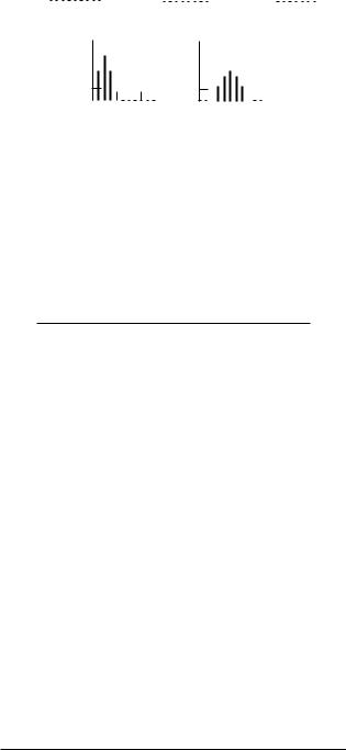
Just after the partition in the box was removed, the situation was very ordered. The system spontaneously approached a much more random situation in which nearly half the molecules were in each half of the box. The actual number n fluctuates about N/2, but in such a way that the average n (taken, say, over several seconds) no longer changes with time. Typical fluctuations with a constant n are shown in Fig. 3.4(a). When the average3

3There is a subtlety about the meaning of average that we are glossing over here. If we take a whole ensemble of identical systems, which were all prepared the same way, and measure n in each one, we have the ensemble average n¯. This is calculated in the way described in Appendix G. If we watch one system over some long time interval, as in Fig. 3.4, we can take the time average n . It is taken by recording values of n for a large number of discrete times in some interval. Strictly speaking, an equilibrium state is one in which the ensemble average is not changing with time.

FIGURE 3.4. (a) Fluctuations of n about N/2. (b) The approach of the system to the equilibrium state after the partition is removed.

of the macroscopic parameters is not changing with time, we say that the system is in an equilibrium state. Figure 3.4(b) shows the system moving toward the equilibrium state after the partition is removed.

An equilibrium state is characterized by macroscopic parameters whose average values remain constant with time, although the parameters may fluctuate about the average value. It is also the most random (i.e., most probable) macrostate possible under the prescribed conditions. It is independent of the past history of the system and is specified by a few macroscopic parameters.4

The definition of a microstate of a system has so far been rather vague; we have not said precisely what is required to specify it. It is actually easier to specify the microstate of a system when using quantum mechanics than when using classical mechanics. When the energy of an individual particle in a system (such as one of the molecules in the box) is measured with su cient accuracy, it is found that only certain discrete values of the energy occur. This is because of the wave nature of the particles. The allowed values of the energy are called energy levels. You are probably familiar with the idea of energy levels from a previous physics or chemistry course; for example, the spectral lines of atoms are due to the emission of light when an atom changes from one energy level to another. Because the energy levels are well defined, the energy di erence, and hence the frequency or color of the light, is also well defined (see Chapter 14).

A particle in a box has a whole set of energy levels at energies determined by the size and shape of the box. Compared to macroscopic measurements of energy, these levels are very close together. The particle can be in any one of these levels; which energy the particle has is specified by a set of quantum numbers. If the particle moves in three dimensions, three quantum numbers are needed

4A more detailed discussion of equilibrium states is found in Reif (1964).

to specify the energy level. If there are N particles, it will be necessary to specify three quantum numbers for each particle or 3N numbers in all. (If there are M molecules, each made up of a atoms, then N = aM . The number of quantum numbers is less than 3N because the atoms cannot all move independently. If the molecules were thought of as single particles, there would be 3M quantum numbers. But the molecules can rotate and vibrate, so that the number of quantum numbers is greater than 3M and less than 3N .)

The total number of quantum numbers required to specify the state of all the particles in the system is called the number of degrees of freedom of the system, f .

A microstate of a system is specified if all the quantum numbers for all the particles in the system are specified.

In most of this chapter, it will not be necessary to consider the energy levels in detail. The important fact is that each particle in a system has discrete energy levels, and a microstate is specified if the energy level occupied by each particle is known.

3.3The Energy of a System: The First Law of Thermodynamics

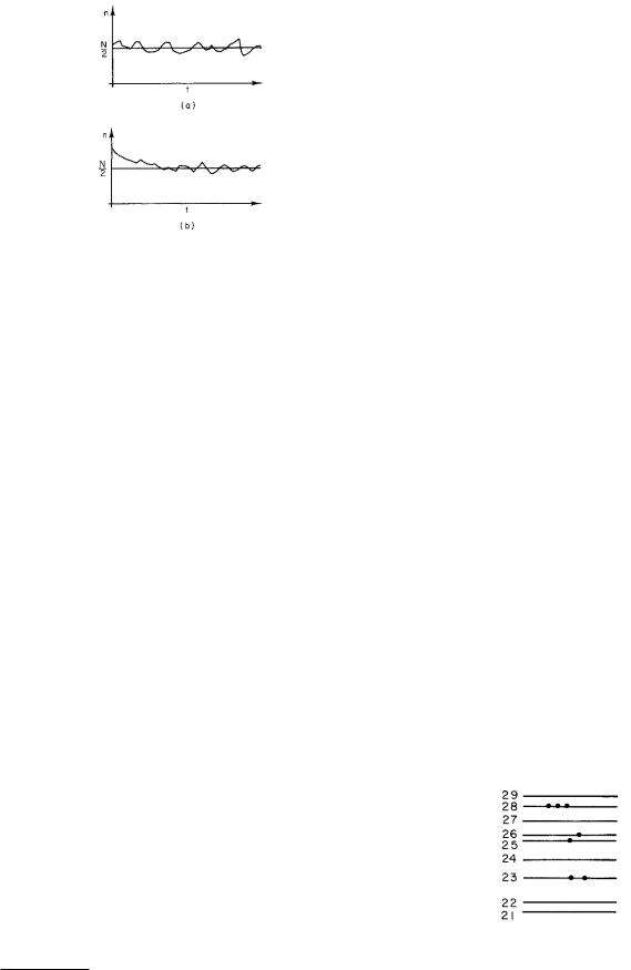
Figure 3.5 shows some energy levels in a system occupied by a few particles. The total energy of the system U is the sum of the energy of each particle. In making this drawing, we have assumed that all the particles are the same and that they do not interact with one another very much. Then each particle has the same set of energy levels, and the presence of other particles does not change them. In that case, we can say that there is a certain set of energy levels in the system and that each level can be occupied by any number of particles. The energy of the ith level, occupied or not, will be called ui. For the example of Fig. 3.5, the total energy is

U = 2u23 + u25 + u26 + 3u28.

Suppose that the system is isolated so that it does not gain or lose energy. It is still possible for particles within

FIGURE 3.5. A few of the energy levels in a system. If a particle has a particular energy, a dot is drawn on the level. More than one particle in this system can have the same quantum numbers.