

Intermediate Physics for Medicine and Biology - Russell K. Hobbie & Bradley J. Roth
.pdf22 |
1. Mechanics |
|
|
|
|
|
|
120 |
|
|
|
|
|
|
100 |
|
|
|
|
|
torr |
80 |
|
|
|
|
|
|
|
|
Aortic Valve Opens |
|
||
Pressure, |
40 |
|
|
|
||
|
|
|
|
|
||
|
60 |
|
|
|
|
|
|
|
|
|
|
Contraction |
|
|
20 |
|
|
|
Filling |
|
|
|
|
|
|
|
|
|
0 |
20 |
40 |
60 |
80 |
100 |
|
0 |
|||||
Ventricular Volume, ml
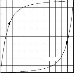
FIGURE 1.35. Pressure–volume relationship in the left ventricle. The curve is traversed counterclockwise with increasing time. The stroke volume is 100 −35 = 65 ml. Systolic pressure is 118 torr, and diastolic pressure is 70 torr. The ventricular pressure drops below diastolic while the pressure in the arteries remains about 70 torr because the aortic valve has closed and prevents back flow
flow: (1) there may be turbulence; (2) there are departures from a parabolic velocity profile; (3) the vessel walls are elastic; and (4) the apparent viscosity depends on the both fraction of the blood volume occupied by red cells and on the size of the vessel.
The importance of turbulence (nonlaminar) flow is determined by a dimensionless number characteristic of the system called the Reynolds number NR. It is defined by
NR = |
LV ρ |
, |
(1.61) |
|
η |
||||
|
|
|
where L is a length characteristic of the problem, V a velocity characteristic of the problem, ρ the density, and η the viscosity of the fluid. When NR is greater than a few thousand, turbulence usually occurs.
The Reynolds number arises in the following way. If we were to write Newton’s second law for a fluid (which we have not done) in terms of dimensionless primed variables such as r = r/L, v = v/V , and t = t/(L/V ), we would find that the equations depend on the properties of the fluid only through the combination NR [Mazumdar (1992), p. 14]. With appropriate scaling of dimensions and times, flows with the same Reynolds number are identical.
There is ambiguity in defining the characteristic length and the characteristic velocity. Should one use the radius or the diameter of a tube? The maximum velocity or the average velocity? If one is solving the equations of motion, one knows what values of L and V were used to transform the equations. They are used to transform the solution back to “real world” coordinates. However, if one is making a statement such as “turbulence usually occurs for values of NR greater than a few thousand,” there is ambiguity. On the other hand, the statement is
not very precise. Sometimes an additional subscript is used to specify how NR was determined.
When NR is large, inertial e ects are important. External forces accelerate the fluid. This happens when the mass is large and the viscosity is small. As the viscosity increases (for fixed L, V , and ρ) the Reynolds number decreases. When the Reynolds number is small, viscous e ects are important. The fluid is not accelerated, and external forces that cause the flow are balanced by viscous forces. Since viscosity is a form of internal friction in the fluid, work done on the system by the external forces is transformed into thermal energy. The low-Reynolds- number regime is so di erent from our everyday experience that the e ects often seem counterintuitive. They are nicely described by Purcell (1977).
Here is an example of an estimate expressed in terms of the Reynolds number. A pressure di erence ∆p acts on a segment of fluid of length ∆x undergoing Poiseuille flow. The di erence between the force exerted on the segment of fluid by the fluid “upstream” and that exerted by the fluid “downstream” is πRp2∆p. If the average speed of the fluid is v, then the net work done on the segment by the fluid upstream and downstream in time ∆t is Wvisc = πRp2∆pv∆t. Since the fluid is not accelerated, this work is converted into thermal energy. We can solve Eq. 1.40 for ∆p and use Eq. 1.43 to write
Wvisc = πRp2 ∆p v∆t = 8ηπv2 ∆x ∆t.
The kinetic energy of the moving fluid in a cylinder of length v∆t is
mv2 |
|
ρ πRp2 ( |
|
∆t) |
|
2 |
|
ρ πRp2 |
|
3 ∆t |
||
= |
v |
v |
= |
v |
||||||||
Ek = |
|
|
|
|
|
|
|
, |
||||
|
|
|
|
|
|
|
||||||
2 |
2 |
|
|
|
|
2 |
|
|
||||
and the ratio of the kinetic energy to the work done is
Ek |
|
|
ρ |
|
Rp2 |
|
1 ρ |
|
Rp |
1 |
|
|||
|
v |
|||||||||||||
|
|
|
v |
|||||||||||
|
= |
|
|
|
|
= |
|
|
|
|
|
= |
|
NR. |
Wvisc |
16η ∆x |
16ξ η |
|
|||||||||||
|
|
|
16ξ |
|||||||||||
(The last step was done by writing the ∆x as ξRp.) This result shows that the ratio of kinetic energy to viscous work is proportional to the Reynolds number. Another example is given in the problems.
A large range of values of NR occurs in the circulatory system. Typical values corresponding to the peak flow are given in Table 1.4. Blood flow is laminar except in the ascending aorta and main pulmonary artery, where turbulence may occur during peak flow.
There are two main causes of departures from the parabolic velocity profile. First, a red cell is about the same diameter as a capillary. Red cells in capillaries line up single file, each nearly blocking the capillary. The plasma flows in small volumes between each red cell, with a velocity profile that is nearly independent of radius. Second, the entry region causes deviations from Poiseuille flow in larger vessels.
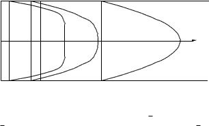
_ |
v/ v |
x = 0 |
x = 20 |
x = 240 |
x = 70 |
FIGURE 1.36. Velocity profiles in steady laminar flow at the entrance to a tube, showing the development of the parabolic velocity profile. The velocity is given as v/v. At the entrance v/v = 1. When the Poiseuille flow is fully developed, v/v is 2 at the center of the tube. These curves are calculated from a graph by Cebeci and Bradshaw (1977) for laminar flow in a tube of radius 2 mm and a pressure gradient of 20 torr m−1, carrying a fluid with a viscosity of 3 × 10⁻³ N s m−2 and a density of 103 kg m−3. The scales are di erent along the axis and radius of the tube; the tube radius is 2 mm and the entrance region is 240 mm long.
Suppose that blood flowing with a nearly flat velocity profile enters a vessel, as might happen when blood flowing in a large vessel enters the vessel of interest, which has a smaller radius. At the wall of the smaller vessel the flow is zero. Since the blood is incompressible, the average velocity is the same at all values of x, the distance along the vessel. (We assume the vessel has constant cross-sectional area.) However, the velocity profile v(r) changes with distance x along the vessel. At the entrance to the vessel (x = 0) there is a very abrupt velocity change near the walls. As x increases a parabolic velocity profile is attained. The transition or entry region, is shown in Fig. 1.36. In the entry region the pressure gradient is di erent from the value for Poiseuille flow. The velocity profile cannot be calculated analytically in the entry region. Various numerical calculations have been made, and the results can be expressed in terms of scaled variables [see, for example, Cebeci and Bradshaw (1977)]. The Reynolds number used in these calculations was based on the diameter of the pipe, D = 2Rp, and the average velocity. The length of the entry region is
L = 0.05DNR,D = 0.1RpNR,D = 0.2RpNR,Rp . (1.62)
Blood pressure is, of course, pulsatile. This means that the average velocity and v(r) are changing with time and also departing from the parabolic profile. Also, at the peak pressure during systole, the aorta and arteries expand, storing some of the blood and releasing it gradually during the rest of the cardiac cycle. Pulsatile flow and the elasticity of vessel walls are discussed extensively by Caro et al. (1978) and by Milnor (1989).
Blood is not a Newtonian fluid. The viscosity depends strongly on the fraction of volume occupied by red cells (the hematocrit). In blood vessels of less than 100 µm radius, the apparent viscosity decreases with tube radius.
Symbols Used |
23 |
Since a red cell barely fits in a capillary, the velocity profile in capillaries is not parabolic. Flow in arterioles and arteries is often modeled as individual particles surrounded by plasma and transported by laminar flow, each red cell staying at its own distance from the central axis. However, high-speed motion pictures show that the red cells often collide with other red cells and with the wall. [See the articles by Trowbridge (1982, 1983) and Trowbridge and Meadowcroft (1983), and also the Caro et al. and Milnor articles.]
Symbols Used in Chapter 1
Symbol |
Use |
Units |
First |
|
|
|
used on |
|
|
|
page |
a, a |
Acceleration |
m s−2 |
3 |
a, b |
Small distances |
m |
13 |
c |
Constant of integration |
|
14 |
g |
Acceleration due to gravity |
m s−2 |
14 |
h |
Small distance |
m |
13 |
i |
Total volume flux or flow |
m3 s−1 |
16 |
|
rate or current |
|
|
jv |
Volume fluence rate or flux |
m s−1 |
16 |
|
density (flow of volume per |
|
|
|
unit area per second) |
|
|
l |
Length of rod |
m |
12 |
m |
Mass |
kg |
3 |
p |
Pressure |
Pa |
13 |
pt |
Pressure in thorax |
Pa |
19 |
pa |
Pressure in alveoli |
Pa |
19 |
r |
Position |
m |
5 |
r |
Distance from origin |
m |
4 |
|
(radius) in polar |
|
|
|
coordinates |
|
|
s |
Displacement |
m |
11 |
sn |
Normal stress |
Pa |
12 |
ss |
Shear stress |
Pa |
13 |
s |
Distance along a streamline |
m |
18 |
t |
Time |
s |
10 |
v, v |
Velocity |
m s−1 |
10 |
x, y, z |
Coordinates |
m |
4 |
xˆ, yˆ, ˆz |
Unit vectors along the x, y, |
|
6 |
|
and z axes |
|
|
A |
Constant of integration |
|
16 |
dA |
Small area perpendicular |
m2 |
18 |
|
to a streamline |
|
|
D |
Pipe diameter |
m |
23 |
E |
Young’s modulus |
Pa |
12 |
Ek |
Kinetic energy |
J |
10 |
F, F |
Force |
N |
3 |
G |
Shear modulus |
Pa |
13 |
L |
Characteristic length |
m |
23 |
N, N |
Force |
N |
7 |
NR |
Reynolds number |
|
22 |
NR,D |
Reynolds number based on |
|
23 |
|
diameter |
|
|
NR,Rp |
Reynolds number based on |
|
23 |
|
pipe radius |
|
|
P |
Power |
W |
11 |
R, R |
Force |
N |
7 |
24 |
1. |
Mechanics |
|
|
Symbol |
|
Use |
Units |
First |
|
|
|
|
used on |
|
|
|
|
page |
Rp |
|
Radius of pipe |
m |
16 |
R |
|
Vascular resistance |
Pa m−3 s |
20 |
S |
|
Cross-sectional area |
m2 |
12 |
V |
|
Volume |
m3 |
15 |
V |
|
Velocity |
m s−1 |
22 |
W, W |
|
Weight |
N |
4 |
W |
|
Work |
J |
19 |
δ |
|
A small distance |
m |
13 |
n |
|
Normal strain |
|
12 |
s |
|
Shear strain |
|
13 |
η |
|
Viscosity |
Pa s |
15 |
α, β, θ, φ |
Angle |
|
5 |
|
κ |
|
Compressibility |
Pa−1 |
15 |
ρ |
|
Mass density |
kg m−3 |
14 |
τ ,τ |
|
Torque |
N m |
4 |
ξ |
|
Dimensionless ratio |
|
22 |
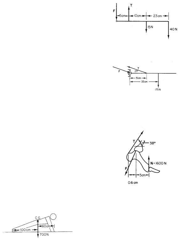
Problem 6 A person with upper arm vertical and forearm horizontal holds a mass of 4 kg. The mass of the forearm is 1.5 kg. Consider four forces acting on the forearm: F by the bones and ligaments of the upper arm at the elbow, T by the biceps, 40 N by the mass, and 15 N as the weight of the arm. The points of application are shown in the drawing. Calculate the vertical components of F and T.
Problems
Section 1.1
Problem 1 Estimate the number of hemoglobin molecules in a red blood cell. Red blood cells are little more than bags of hemoglobin, so it is reasonable to assume that the hemoglobin takes up all the volume of the cell.
Problem 2 Our genetic information or genome is stored in the parts of the DNA molecule called base pairs. Our genome contains about 3 billion 3 × 10⁹ base pairs, and there are two copies in each cell. Along the DNA molecule, there is one base pair every one-third of a nanometer. How long would the DNA helix from one cell be if it were stretched out in a line? If the entire DNA molecule were wrapped up into a sphere, what would be the diameter of that sphere?
Problem 3 Estimate the size of a box containing one air molecule. (Hint: What is the volume of one mole of gas at standard temperature and pressure?) Compare the size of the box to the size of an air molecule (about 0.1 nm).
Problem 4 Estimate the density of water (H2O) in kg m−3. Useful information: an oxygen atom contains 8 protons and 8 neutrons. A hydrogen atom contains 1 proton and no neutrons. The mass of the electron is negligible.
Problem 7 When the arm is stretched out horizontally, it is held by the deltoid muscle. The situation is shown schematically. Determine T and F.
Section 1.5
Problem 8 When a person crouches, the geometry of the heel is as shown. Determine T and F. Assume all the forces act in the plane of the drawing.
Section 1.3
Problem 5 A person with mass m = 70 kg has a weight (mg) of about 700 N. If the person is doing push-ups as shown, what are the vertical components of the forces exerted by the floor on the hands and feet?
Problem 9 A person of weight W is suspended by both hands from a high bar as shown. The center of mass is directly below the bar.
(a)Find the horizontal and vertical components Fx and Fy , where F is the force exerted by the bar on each of the two hands.
(b)Given the additional information about the arm shown in the second drawing, calculate the components of R, the force exerted by the humerus on the forearm through the elbow, and the tension T in the biceps tendon. Neglect the weight of the arm, and assume that T
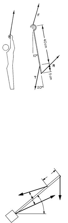
and R are the only forces exerted on the forearm by the upper arm.
Problems 25
Section 1.7
Problem 11 Suppose that instead of using a cane, a person holds a suitcase of weight W/4 in one hand, 0.4 m from the midline. The person is standing on the opposite leg. Calculate the force exerted by the hip abductor muscles and by the acetabulum on that leg.
Problem 10 Consider the forces on the spine when lifting. Approximate the spinal column as a sti bar of length L that has three forces acting on it. W is the downward force acting at the top of the spinal column (via the arms and shoulders), and equals the weight of the object being lifted. F is the force applied by the erector spinae muscle, which attaches to the spine about one-third of the way from the top of the column. Assume this muscle acts at an angle of 12 ◦ to the spinal column. R is the force the pelvis exerts on the spinal column. The weight of the trunk is neglected. Assume the spinal column makes an angle θ with the horizontal.
L/3
Spine
F
12¡
 φ θ R W
Pelvis
Section 1.9
Problem 12 Young’s modulus for a spider’s thread is about 0.2 ×10¹⁰ Pa, and the thread breaks when it undergoes a strain of about 50% [K¨ohler and Vollrath (1995)].
(a)Calculate the tensile strength of the thread and compare it to the tensile strength of steel.
(b)Calculate the strain that steel undergoes when it breaks. (Assume that a linear relationship between stress and strain holds until it breaks.) Compare the breaking strain to the spider’s thread.
Problem 13 Assume an object undergoes a normal strain in all three directions: x = ∆x/lx, y = ∆y/ly ,z = ∆z/lz . Relate the three strains to the change in volume of the object. Assume the strains are small.
Section 1.10
Problem 14 Relate the shear strain to angle θ in Fig. 1.23. How does this relationship simplify if θ is small?
Section 1.11
Problem 15 The inspirational pressure di erence pin that the lung can generate is about 86 torr. What would be the absolute maximum depth at which a person could breathe through a snorkel device? (A safe depth is only about half this maximum, since the lung ventilation becomes very small at the maximum depth. Assume the lungs are 30 cm below the mouth.)
Problem 16 A person standing erect can in some cases be modeled by a column of water.
(a)Calculate the hydrostatic pressure di erence between a person’s head and foot in torr.
(b)Explain why blood pressure is measured in the arm at the same vertical height as the heart.
(c)Our body has adapted to having a larger hydrostatic pressure in our feet than in our head. Speculate on why you feel uncomfortable when you “stand on your head.”
(a)Determine R and F in terms of W and θ.
(b)The spinal column may be injured if R is too large. Problem 17 A medication dissolved in a saline solution
Compare R when θ is 0 ◦ and 90 ◦. This problem explains why people say to “lift with your legs, not with your back.”
(c) Compare the angle φ when θ is 0 ◦ and 90 ◦ . If φ is not close to zero, there will be considerable transverse force at the disks in the lower back, which is not a good situation.
is infused into a vein in the patients arm (IV infusion). The density of saline is the same as water. The pressure of the blood inside the vein is 5 torr above atmospheric pressure. How high above the insertion point must the container be hung so that there is su cient hydrostatic pressure to force fluid into the vein?
26 1. Mechanics
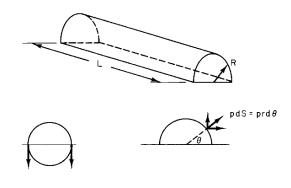
Problem 18 The walls of a cylindrical pipe that has an excess pressure p inside are subject to a tension force per unit length T . (Consider only the force per unit length in the walls of the cylinder, not the force in any end caps of the pipe.) The force per unit length in the walls can be calculated by considering a di erent pipe made up of two parts as shown in the figure: a semicircular half-cylinder of radius R and length L attached to a flat plate of width 2R and length L. What is the force that the excess pressure exerts on the flat plate? Show that the tension force per unit length in the wall of the tube is f = pR. This is called the Law of Laplace. (Do not worry about any deformation.)
See if you can obtain the same answer by direct integration of the horizontal and vertical components of the force due to the excess pressure.
Sometimes a patient will have an aneurysm in which a portion of an artery will balloon out and possibly rupture. Comment on this phenomenon in light of the R dependence of the force per unit length [Hademenos (1995)].
Problem 19 Find a relationship among the tension per unit length T across any element of the wall of a soap bubble, the excess pressure inside the bubble, ∆p, and the radius of the bubble, R. (Hint: Use the same technique as for the previous problem.)
Section 1.12
Problem 20 Suppose a fish has an average density of 1030 kg m−3, compared to the density of the surrounding water, 1000 kg m−3. One way the fish can keep from slowly sinking is by using an air bladder (the density of air is 1.2 kg m−3). What fraction of the fish’s total volume must be air in order for the fish to be neutrally buoyant (the buoyant force is equal and opposite to the weight). Assume that the volume V of the fish’s tissue is fixed, so in order to increase the volume U of the air bladder, the total volume of the fish V + U must increase.
Problem 21 This problem explores the physics of a centrifuge. A cylinder of fluid of density ρfluid and length L is rotated at an angular velocity ω (rad s−1) in a horizontal plane about a vertical axis through one end of the tube. Neglect gravity. An object moving in a circle with
constant angular velocity has an acceleration a = −rω2 toward the center of the circle. Find the pressure in the fluid as a function of distance from the axis of rotation, assuming the pressure is p0 at r = 0.
Problem 22 Buoyancy plays an important role in the centrifuge. Consider a small cubic particle of density ρ immersed in a fluid of density ρfluid.
(a) Write Newton’s second law for the particle, considering only the centripetal acceleration and the pressure exerted by the fluid (Problem 21). Find an expression for the “e ective weight” of the particle (analogous to Eq. 1.31) in terms of ρ, ρfluid, ω, r, and the particle volume V . Your result is more general than you might expect: it is true for a particle of any shape [Wick and Tooby (1977)].
(b)Find the ratio of the “e ective weight” derived in
(a)to the “e ective weight” due to gravity (Eq. 1.31).
(c)If the particle is 10 cm from the axis of a centrifuge spinning at 40 000 revolutions per minute, evaluate the ratio obtained in (b).
(d)The “density gradient” technique uses a sucrose solution of varying concentration to produce a fluid density
that varies with r, ρfluid(r). Explain how in this case the centrifuge can be used to separate particles of di erent densities.
Problem 23 For the centrifuge of Problem 22 assume there is one additional force: a viscous force proportional to the speed u of the particle relative to the fluid.
(a)Derive an expression for u, the “sedimentation velocity” assuming the particle is not accelerating relative to the fluid.
(b)The sedimentation velocity per unit acceleration, S, is a parameter commonly used in centrifuge work. Divide the expression obtained in (a) by the centripetal accelera-
tion to obtain an expression for S. The common unit for
Sis the svedberg (1 Sv = 10−13 s).
(c)Consider two particles with S = 50 and 70 Sv. For the centrifuge of Problem 22(c), how long will it take for the particles to separate by 3 mm if they were initially at the same position? How long would this separation take if gravity were used instead of a centrifuge?
Section 1.13
Problem 24 What is the compressibility of a gas for which pV =const? Compare the compressibility of water to that of air at atmospheric pressure. What are the implications of this for the volume of the lungs of a swimmer diving deep below the water surface?
Problem 25 Figure 1.20, showing a rod subject to a force along its length, is a simplification. Actually, the cross-sectional area of the rod shrinks as the rod lengthens. Let the axial strain and stress be along the z axis. They are related by Eq. 1.25, sz = E z . The lateral strains x and y are related to sz by sz = −(E/ν) x =
−(E/ν) y ,where ν is called the “Poisson’s ratio” of the material.
(a)Use the result of Problem 13 to relate E and ν to the fractional change in volume ∆V /V .
(b)The change in volume caused by hydrostatic pressure is the sum of the volume changes caused by axial stresses in all three directions. Relate Poisson’s ratio to the compressibility.
(c)What value of ν corresponds to an incompressible material?
(d)For an isotropic material, −1 < ν < 0.5. How would a material with negative ν behave?
Elliott et al. (2002) measured Poisson’s ratio for articular (joint) cartilage under tension and found 1 < ν < 2. This large value is possible because cartilage in anisotropic: its properties depend on direction.
Problems 27
Section 1.15
Problem 30 Consider laminar flow in a pipe of length ∆x and radius Rp. Find the total viscous drag exerted by the pipe on the fluid.
Problem 31 The maximum flow rate from the heart is 500 ml s−1. If the aorta has a diameter of 2.5 cm and the flow is Poiseuille, what are the average velocity, the maximum velocity at the center of the vessel, and the pressure gradient along the vessel? Plot the velocity vs distance from the center of the vessel. As an approximation to the viscosity of blood, use η = 10−3 kg m−1 s−1.
Problem 32 The glomerular pore described in Eq. 1.41 has a flow i = 7.2 × 10⁻²¹ m3 s−1. How many molecules of water per second flow through it? What is their average speed?
Problem 33 A parent vessel of radius Rp branches into two daughter vessels of radii Rd1 and Rd2. Find a relationship between the radii such that the shear stress on the vessel wall is the same in each vessel. (Hint: Use conservation of the volume flow.) This relationship is called “Murray’s Law”. Organisms may use shear stress to determine the appropriate size of vessels for fluid transport [LaBarbera (1990)].
Problem 27 Consider fluid flowing between two slabs as |
|
|
shown in Fig. 1.26. Since the work done by the external |
Problem 34 Sap flows up a tree at a speed of about 1 |
|
force on the system in time dt is dW = F vdt, the rate |
||
of doing work is P = dW/dt = F v, where v is the speed |
mm s−1 through its vascular system (xylem), which con- |
|
of the moving plate. Find the power dissipated per unit |
sists of cylindrical pores of 20 µm radius. Assume the vis- |
|
volume of the fluid in terms of the velocity gradient. |
cosity of sap is the same as the viscosity of water. What |
|
Problem 28 Consider a fluid that is flowing in the x |
pressure di erence between the bottom and top of a 100 |
|
m tall tree is needed to generate this flow? How does it |
||
direction, but with the velocity vx changing in the y di- |
||
compare to the hydrostatic pressure di erence caused by |
||
rection. |
||
gravity? |
||
(a) Start with Newton’s second law. Analyze the forces |
||
|
||
on a small cube of fluid and derive the equation |
|
|
∂vx |
∂vx |
|
∂p |
|
∂2vx |
|||
ρ |
|
+ ρvx |
|
= − |
|
|
+ η |
|
. |
∂t |
∂x |
∂x |
∂y2 |
||||||
This is a simplified version of the Navier-Stokes equation that governs fluid flow.
(b) Which term in the equation is nonlinear (that is, if p and vx are doubled, which term does not double)? A nonlinear equation is needed to describe complicated flows such as turbulence.
Problem 29 Consider the simplified version of the Navier-Stokes equation in Problem 28. Assume the fluid speed is approximately V and all spatial changes occur over distances of order L. Take the ratio of the “inertial term” ρvx(∂vx/∂x) to the “viscous term” η(∂2vx/∂y2) and show that you get the Reynolds number, Eq. 1.61.
Problem 35 Consider a small cube of incompressible fluid. Analyze the volume fluence rate for each face of the cube and show that the divergence of v is zero. (The divergence is defined in Chapter 4.)
Section 1.16
Problem 36 The accompanying figure shows the negative pressure (below atmospheric) that must be maintained in the thorax during the respiratory cycle by a patient with airway obstruction in order to breathe. Viscous e ects are included. Estimate the work in joules done by the body during a breath.
28 |
|
1. |
Mechanics |
|
|
|
|
|
|
|
|
-6.0 |
|
|
|
|
|
|
|
|
|
|
|
|
Inspiration |
|
|
||
|
O) |
|
|
|
|
|
|
|
|
|
2 |
|
|
|
|
|
|
|
|
|
(cm H |
|
|
|
|
|
|
|
|
|
Pressure |
-5.0 |
|
|
|
|
|
|
|
|
|
|
|
|
|
|
|
|
|
|
|
|
|
|
|
|
Expiration |
|
|
|
- |
|
|
|
|
|
|
|
|
|
|
-4.0 |
|
0.1 |
0.2 |
0.3 |
0.4 |
0.5 |
0.6 |
|
|
0.0 |
|||||||
|
|
|
|
|
Volume change (liters) |
|
|
||
Section 1.17
Problem 37 The volume of blood in a typical person is 5 liters, and the volume current through the aorta is about
5liter min−1.
(a)What is the total volume current through all the systemic capillaries?
(b)What is the total volume current through all the pulmonary capillaries?
(c)How long does the blood take to make one complete circuit through the circulatory system?
Problem 38 Find the conversion factor between PRU and Pa m−3 s.
Problem 39 Equation 1.58 relates the resistance of a vessel to its radius. In the circulatory system, the resistance of an arteriole increases when the smooth muscle surrounding the arteriole contracts, thereby decreasing its radius. By what factor does the resistance increase if the radius decreases by 10%?
Problem 40 Derive the equations for resistance in a collection of vessels in series and in parallel. Remember that when several vessels are in series, the current is constant and the total pressure change is the sum of the pressure changes along the length of each vessel. When vessels are in parallel, each has the same pressure drop, but the current before the vessels branch is the sum of the currents in each branch.
Problem 41 The velocity of the blood in the aorta is about 0.5 m s−1, and the velocity of the blood in a capillary is about 0.001 m s−1. We have only one aorta, with a diameter of 20 mm, but many capillaries in parallel, each with a diameter of 8 µm. Estimate how many capillaries are typically open at any one time.
Problem 42 Suppose a student asked you, “How can blood be moving more slowly in a capillary than in
the aorta? For an incompressible fluid, when the crosssectional area along a pipe decreases, the velocity increases, so that the volume current i is the same. The capillary has a much smaller cross-sectional area than the aorta. Therefore, the blood should move faster in the capillary than in the aorta!” How would you respond to this student?
Problem 43 For Poiseuille flow, find an expression for the maximum shear rate in each vessel from Eq. 1.44. Where in the vessel does it occur? Typical maximum shear rates are 50 s−1 in the aorta, 150 s−1 in the femoral artery, and 400 s−1 in an arteriole.
Problem 44 A sphere of radius a moving through a fluid with speed v is subject to a viscous drag Fdrag = 6πηav. Make an argument similar to that in the text to show that the ratio of kinetic energy of a sphere of fluid of the same size moving at the same speed to the viscous work done to displace the sphere by its own diameter is NR/18.
Problem 45 Find an expression for the entry length in terms of the tube size, the pressure gradient, and the properties of the fluid. Estimate the length of the entry region in the aorta, in an artery, and in an arteriole of radius 20 µm. Use η = 10−3 kg m−1 s−1.
Problem 46 Estimate the tension per unit length and the stress in the walls of various blood vessels using the data in Table 1.4.
Problem 47 Consider laminar viscous flow in the following situation, which models flow in the bronchi or a network of branching blood vessels. A vessel of radius R connects to N smaller vessels, each of radius xR.
(a)What is the relationship between total crosssectional area of the smaller vessels and that of the larger vessel if the pressure gradient is the same in both sets of vessels?
(b)How do the pressure gradients compare if the total cross-sectional area is the same in both sets of vessels? (Neither assumption is realistic.)
Problem 48 Compare the magnitude of the four terms in Eq. 1.42 in the following two cases. Ignore branching. Assume the vessels are vertical. Use ρ = 103 kg m−3 and
η= 10−3 Pa s.
(a)The descending aorta. Assume the length is 35 cm,
the radius is 1 cm (independent of distance along the aorta), the peak acceleration of the blood is 1800 cm s−2,
and the peak velocity (during the cardiac cycle) is 70 cm s−1 at the entrance and 60 cm s−1 at the exit. (These velocities are di erent because some of the blood leaves the aorta in major arteries.)
(b)An arteriole of radius 50 µm, length 1 mm, and constant velocity of 5 mm s−1 at both entrance and exit.
Problem 49 The viscosity of water (and therefore of blood) is a rapidly decreasing function of temperature.
Water at 5 ◦C is twice as viscous as water at 35 ◦C. Speculate on the implications of this extreme temperature dependence for the circulatory system of cold-blooded animals. [For a further discussion see Vogel (1994), pp. 27– 31.]
Section 1.18
Problem 50 Estimate the Reynolds number for the following flows. In each case, determine whether the Reynolds number is high ( 1) or low ( 1).
(a)E. coli bacteria (length 2 microns) swim in water at speeds of about 0.01 mm s−1.
(b)An Olympic swimmer (length 2 m) swims in water at speeds of up to 2 m s−1.
(c)A bald eagle (wingspan = 2 m) flies in air (density = 1.2 kg m−3, viscosity = 1.8 × 10⁻⁵ Pa s) at speeds of 20 km hr−1.
Problem 51 Estimate the Reynolds number of blood flow in a capillary, using the data in Table 1.4. How does this compare to that in the aorta?
References
Benedek, G. B., and F. M. H. Villars (2000). Physics with Illustrative Examples from Medicine and Biology. Vol. 1.
Mechanics. New York, Springer-Verlag.
Caro, C. G., T. J. Pedley, R. C. Schroter, and W. A. Seed (1978). The Mechanics of the Circulation. Oxford, Oxford University Press.
Cebeci, T., and P. Bradshaw (1977). Momentum Transfer in Boundary Layers. Washington, Hemisphere.
Denny, M. W. (1993). Air and Water: The Biology and Physics of Life’s Media. Princeton, Princeton University Press.
Elliott, D. M., D. A. Normoneva and L. A. Setton (2002). Direct measurement of the Poisson’s ratio of human patella cartilage in tension. J. Biomech. Eng. 124: 223–228.
Fung, Y. C. (1993). Biomechanics: Mechanical Properties of Living Tissue. 2nd. ed. New York, SpringerVerlag.
Goodsell, D. S. (1998). The Machinery of Life. New York, Springer-Verlag.
Hademenos, G. J. (1995). The physics of cerebral aneurysms. Physics Today, Feb., 24-30.
Halliday, D., R. Resnick, and K. S. Krane (1992). Fundamentals of Physics, 4th ed., Vol. 1. New York, Wiley.
References 29
Herrick, J. F. (1942). Poiseuille’s observations on blood flow lead to a new law in hydrodynamics. Am. J. Phys. 10: 33–39.
Inman, V. T. (1947). Functional aspects of the abductor muscles of the hip. J. Bone Joint Surg. 29: 607–619.
K¨ohler, T. and F. Vollrath (1995). Thread biomechanics in the two orb-weaving spiders, Araneus diadematus (Araneae, Araneidae) and Uloborus walckenaerius
(Araneae, Uloboridae). J. Exp. Zool. 271: 1–17. LaBarbera, M. (1990). Principles of design of fluid
transport systems in zoology. Science. 249: 992–1000. Lighthill, J. (1975). Mathematical Biofluiddynamics.
Philadelphia, Society for Industrial and Applied Mathematics.
Macklem, P. T. (1975). Tests of lung mechanics. N. Engl. J. Med. 293: 339–342.
Mazumdar, J. N. (1992). Biofluid Mechanics. Singapore, World Scientific.
Milnor, William R. (1989). Hemodynamics, 2nd ed. Baltimore, Williams & Wilkins.
Morrison, P., P. Morrison, and the o ce of C. & R. Eames (1994). Powers of Ten. New York, Scientific American Library.
Patton, H. D., A. F. Fuchs, B. Hille, A. M. Scher and R. Steiner, eds. (1989). Textbook of Physiology. 21st ed. Philadelphia, Saunders.
Purcell, E. M. (1977). Life at low Reynolds number.
Am. J. Phys. 45: 3–11.
Synolakis, C. E., and H. S. Badeer (1989). On combining the Bernoulli and Poiseuille equation—A plea to authors of college physics texts. Am. J. Phys. 57(11): 1013–1019.
Trowbridge, E. A. (1982). The fluid mechanics of blood: equilibrium and sedimentation. Clin. Phys. Physiol. Meas. 3(4): 249–265.
Trowbridge, E. A. (1983). The physics of arteriole blood flow. I. General theory. Clin. Phys. Physiol. Meas. 4(2): 151–175.
Trowbridge, E. A. and P. M. Meadowcroft (1983). The physics of arteriole blood flow. II. Comparison of theory with experiment. Clin. Phys. Physiol. Meas. 4(2): 177– 196.
Vogel, S. V. (1992). Vital Circuits: On Pumps, Pipes, and the Workings of Circulatory Systems. Oxford, Oxford University Press.
Vogel, S. V. (1994). Life in Moving Fluids. Princeton, Princeton University Press.
Wick, G. L. and P. F. Tooby (1977). Centrifugal buoyancy forces. Amer. J. Physics 45: 1074–1076.
Williams, M., and H. R. Lissner (1962). Biomechanics of Human Motion. Philadelphia, Saunders.
2
Exponential Growth and Decay
The exponential function is one of the most important and widely occurring functions in physics and biology. In biology, it may describe the growth of bacteria or animal populations, the decrease of the number of bacteria in response to a sterilization process, the growth of a tumor, or the absorption or excretion of a drug. (Exponential growth cannot continue forever because of limitations of nutrients, etc.) Knowledge of the exponential function makes it easier to understand birth and death rates, even when they are not constant. In physics, the exponential function describes the decay of radioactive nuclei, the emission of light by atoms, the absorption of light as it passes through matter, the change of voltage or current in some electrical circuits, the variation of temperature with time as a warm object cools, and the rate of some chemical reactions.
In this book, the exponential function will be needed to describe certain probability distributions, the concentration ratio of ions across a cell membrane, the flow of solute particles through membranes, the decay of a signal traveling along a nerve axon, and the return of some physiologic variables to their equilibrium values after they have been disturbed.
Because the exponential function is so important, and because we have seen many students who did not understand it even after having been exposed to it, the chapter starts with a gentle introduction to exponential growth (Sec. 2.1) and decay (Sec. 2.2). Section 2.3 shows how to analyze exponential data using semilogarithmic graph paper. The next section shows how to use semilogarithmic graph paper to find instantaneous growth or decay rates when the rate varies. Some would argue that the availability of computer programs that automatically produce logarithmic scales for plots makes these sections unnecessary. We feel that intelligent use of semilogarithmic and logarithmic (log-log) plots requires an understanding of the basic principles.
Variable rates are described in Sec. 2.4. Clearance, discussed in Sec. 2.5, is an exponential decay process that is important in physiology. Sometimes there are competing paths for exponential removal of a substance: multiple decay paths are introduced in Sec. 2.6. A very basic and simple model for many processes is the combination of input at a fixed rate accompanied by exponential decay, described in Sec. 2.7. Sometimes a substance exists in two forms, each with its own decay rate. One then must fit two or more exponentials to the set of data, as shown in Sec. 2.8.
Section 2.9 discusses the logistic equation, one possible model for a situation in which the growth rate decreases as the amount of substance increases. The chapter closes with a section on power-law relationships. While not exponential, they are included because data analysis can be done with log–log graph paper, a technique similar to that for semilog paper. If you feel mathematically secure, you may wish to skim the first four sections, but you will probably find the rest of the chapter worth reading.
2.1 Exponential Growth
An exponential growth process is one in which the rate of increase of a quantity is proportional to the present value of that quantity. The simplest example is a savings account. If the interest rate is 5% and if the interest is credited to the account once a year, the account increases in value by 5% of its present value each year. If the account starts out with $100, then at the end of the first year, $5 is credited to the account and the value becomes $105. At the end of the second year, 5 percent of $105 is credited to the account and the value grows by $5.25 to $110.25. The growth of such an account is shown in Table 2.1 and Fig. 2.1. These amounts can be calculated as follows. At the end of the first year, the original

32 2. Exponential Growth and Decay
TABLE 2.1. Growth of a savings account earning 5% interest compounded annually, when the initial investment is $100.
Year |
Amount |
Year |
Amount |
Year |
Amount |
||
1 |
$105.00 |
10 |
$162.88 |
100 |
$13,150.13 |
||
2 |
110.25 |
20 |
265.33 |
200 |
1,729,258.09 |
||
3 |
115.76 |
30 |
432.19 |
300 |
2.27 × |
108 |
|
|
|
|
|
10 |
|||
4 |
121.55 |
40 |
704.00 |
400 |
2.99 × 10¹² |
||
5 |
127.63 |
50 |
1146.74 |
500 |
3.93 × 10¹⁴ |
||
6 |
134.01 |
60 |
1867.92 |
600 |
5.17 |
× 1016 |
|
7 |
140.71 |
70 |
3042.64 |
700 |
6.80 |
× 1018 |
|
8 |
147.75 |
80 |
4956.14 |
800 |
8.94 |
× 1021 |
|
9 |
155.13 |
90 |
8073.04 |
900 |
1.18 |
× 10 |
|
amount, y0, has been augmented by (0.05)y0:
y1 = y0(1 + 0.5).
During the second year, the amount y1 increases by 5%,
so
y2 = y1(1.05) = y0(1.05)(1.05) = y0(1.05)2.
After t years, the amount in the account is
yt = y0(1.05)t.
In general, if the growth rate is b per compounding period, the amount after t periods is
yt = y0(1 + b)t. |
(2.1) |
It is possible to keep the same annual growth (interest) rate, but to compound more often than once a year. Table 2.2 shows the e ect of di erent compounding intervals on the amount, when the interest rate is 5%. The last two columns, for monthly compounding and for “instant
|
900 |
|
|
800 |
|
|
700 |
|
(dollars) |
600 |
|
500 |
||
Value |
||
400 |
||
|
||
|
300 |
|
|
200 |
|
|
100 |
|
|
0 |
0 |
10 |
20 |
30 |
40 |
50 |
Time (years)
FIGURE 2.1. The amount in a savings account after t years,
TABLE 2.2. Amount of an initial investment of $100 at 5% annual interest, with di erent methods of compounding.
Month |
Annual |
Semiannual |
Quarterly |
Monthly |
Instant |
|
|
|
|
|
|
0 |
$100.00 |
$100.00 |
$100.00 |
$100.000 |
$100.000 |
1 |
100.00 |
100.00 |
100.00 |
100.417 |
100.418 |
2 |
100.00 |
100.00 |
100.00 |
100.835 |
100.837 |
3 |
100.00 |
100.00 |
101.25 |
101.255 |
101.258 |
4 |
100.00 |
100.00 |
101.25 |
101.677 |
101.681 |
5 |
100.00 |
100.00 |
101.25 |
102.101 |
102.105 |
6 |
100.00 |
102.50 |
102.52 |
102.526 |
102.532 |
7 |
100.00 |
102.50 |
102.52 |
102.953 |
102.960 |
8 |
100.00 |
102.50 |
102.52 |
103.382 |
103.390 |
9 |
100.00 |
102.50 |
103.80 |
103.813 |
103.821 |
10 |
100.00 |
102.50 |
103.80 |
104.246 |
104.255 |
11 |
100.00 |
102.50 |
103.80 |
104.680 |
104.690 |
12 |
105.00 |
105.06 |
105.09 |
105.116 |
105.127 |
|
|
|
|
|
|
interest,” are listed to the nearest tenth of a cent to show the slight di erence between them.
The table entries were calculated in the following way. Suppose that compounding is done N times a year. In t years, the number of compoundings is N t. If the annual fractional rate of increase is b, the increase per compounding is b/N . For six months at 5% (b = 0.05) the increase is 2.5, for three months it is 1.25, etc. The amount after t units of time (years) is, in analogy with Eq. 2.1,
y = y0 (1 + b/N )N t . |
(2.2) |
Recall (refer to Appendix C) that (a)bc = (ab)c. The expression for y can be written as
y = y0 |
(1 + b/N )N t . |
(2.3) |
Most calculus textbooks show that the quantity
(1 + b/N )N → eb
as N becomes very large. (Rather than prove this fact here, we give numerical examples in Table 2.3 for two di erent values of b.) Therefore, Eq. 2.3 can be rewritten as
y = y0ebt = y0 exp(bt). |
(2.4) |
(The exp notation is used when the argument is complicated.) To calculate the amount for instant interest, it is necessary only to multiply the fractional growth rate per unit time b by the length of the time interval and then
TABLE 2.3. Numerical examples of the convergence of (1 + b/N )N to eb as N becomes large.
N |
b = 1 |
b = 0.5 |
10 |
2.594 |
1.0511 |
100 |
2.705 |
1.0513 |
1000 |
2.717 |
1.0513 |
eb |
2.718 |
1.0513 |
when the amount is compounded annually at 5% interest.