

Intermediate Physics for Medicine and Biology - Russell K. Hobbie & Bradley J. Roth
.pdf12 1. Mechanics
FIGURE 1.20. A rod subject to a force F along it.
1.9 Stress and Strain
Whenever a force acts on an object, it undergoes a change of shape or deformation. Often these deformations can be ignored, as they were in the previous sections. In other cases, such as the contraction of a muscle, the expansion of the lungs, or the propagation of a sound wave, the deformation is central to the problem and must be considered. This book will not develop the properties of deformable bodies extensively; nevertheless deformable body mechanics is important in many areas of biology [Fung (1993)]. We will develop the subject only enough to be able to consider viscous forces in fluids.
Consider a rod of cross-sectional area S. One end is anchored, and a force F is exerted on the other end parallel to the rod (Fig. 1.20). E ects of weight will be ignored. A surface force is transmitted across any surface defined by an imaginary cut perpendicular to the axis of the rod. A surface force is exerted by the substance to the right of the cut on the substance to the left (and vice versa, in accordance with Newton’s third law: when object A exerts a force on object B, object B exerts an equal and opposite force on object A). The surface force per unit area is called the stress. In this case, when the surface is perpendicular to the axis of the rod and the force is along the axis of the rod, it is called a normal stress:
FIGURE 1.21. A typical stress–strain relationship. On the left, stress is the independent variable. On the right, strain is the independent variable. Strain is usually used as the independent variable because it is often a double-valued function of the stress.
In the linear region, the relationship between stress and strain is written as
sn = E n. |
(1.25) |
The proportionality constant E is called Young’s modulus. Since the strain is dimensionless, E has the dimensions of stress. Various units are N m−2 or pascal (Pa), dyn cm−2, psi (pound per square inch), and bar (1 bar = 14.5 psi = 105 Pa = 106 dyn cm−2).
If the stress is increased enough, the bar breaks. The value of the stress when the bar breaks under tension is called the tensile strength. The material will also rupture under compressive stress; the rupture value is called the compressive strength. Table 1.3 gives values of Young’s modulus, the tensile strength, and the compressive strength for steel, long bone (femur), and wood (walnut).
In some materials, the stress depends not only on the strain, but on the rate at which the strain is produced. It may take more stress to stretch the material rapidly than to stretch it slowly, and more stress to stretch it than
sn = |
F |
. |
(1.23) |
|
|||
|
S |
|
|
In the general case there can also be a component of stress parallel to the surface.
The strain n is the fractional change in the length of the rod:
n = |
∆l |
. |
(1.24) |
|
|||
|
l |
|
|
If increasing stress is applied to a typical substance, the strain increases linearly with the stress for small stresses. Then it increases even more rapidly. At higher strains it may be necessary to reduce the stress to maintain the same strain. Finally, at a high enough strain, the sample breaks. This is plotted in Fig. 1.21. Because of the doublevaluedness of the strain as a function of stress, the strain is usually plotted as the independent variable, as on the right in Fig. 1.21.
TABLE 1.3. Young’s modulus, tensile strength, and compressive strength of various materials in Pa.
Material |
E |
|
|
Tensile |
Compressive |
||||
|
|
|
|
|
strength |
strength |
|||
|
|
|
|
|
|
|
|
|
|
Steel |
(ap20 |
× |
1010 |
50 |
× |
107 |
|
|
|
a |
|
|
|
|
|
|
|||
prox.) |
|
|
|
|
|
|
|
|
|
Femurb |
1.4 × 10¹⁰ |
8.3 × 10⁷ |
1.8 × 10⁷ |
|
|||||
(wet) |
|
0.8 × 10¹⁰ |
4.1 × 10⁷ |
5.2 × 10⁷ |
|
||||
Walnut c |
|
||||||||
aAmerican Institute of Physics Handbook (1957). New York, McGraw-Hill, pp. 2-70.
bB. K. F. Kummer (1972), Biomechanics of bone. In Y. C. Fung, et al. eds., Biomechanics—Its Foundations and Objectives. Englewood Cli s, NJ, Prentice-Hall, p. 237.
cU.S. Department of Agriculture (1955). Wood Handbook, Handbook No. 72. Washington, D.C., U.S. Government Printing O ce, p. 74.

FIGURE 1.22. A pressure–volume curve for a normal lung, showing hysteresis. The elastic recoil pressure is the di erence between the pressure in the alveoli (air sacs) of the lung and the thorax just outside the lung. From P. T. Macklem.Tests of lung mechanics. N. Engl. J. Med. 293: 339–342. Copyrightc 1975 Massachusetts Medical Society. All rights reserved. Drawing courtesy of Prof. Macklem.
to maintain a fixed strain. Such materials are called viscoelastic. They are often important biologically but will not be discussed here [Fung (1993)].
Still other materials exhibit hysteresis. The stress– strain relationship is di erent when the material is being stretched than when it is allowed to return to its unstretched state. This di erence is observed even if the strain is changed so slowly that viscoelastic e ects are unimportant. Figure 1.22 shows a pressure–volume curve for the lung. It is related to the stress–strain relationship for the lung tissue and shows hysteresis.
1.10 Shear
In a shear stress, the force is parallel to the surface across which it is transmitted.6 In a shear strain, the deformation increases as one moves in a direction perpendicular to the deformation. Examples of shear stress and strain are shown in Fig. 1.23. The shear stress is
ss = |
F |
, |
(1.26) |
||
S |
|||||
|
|
|
|||
and the shear strain is |
|
|
|
|
|
s = |
δ |
. |
(1.27) |
||
|
|||||
|
h |
|
|
||
6This discussion of stress and strain has been made simpler than is often the case. In general, the force F across any surface is a vector. It can be resolved into a component perpendicular to the surface and two components parallel to the surface. One can speak of nine components of stress: sxx, sxy , sxz , syx, syy , syz , szx, szy , szz . The first subscript denotes the direction of the force and the second denotes the normal to the surface across which the force acts. Components sxx, syy and szz are normal stresses; the others are shear stresses. It can be shown that sxy = syx, and so forth.
1.10 Shear |
13 |
FIGURE 1.23. Shear stress and strain.
|
|
|
|
|
|
|
|
|
|
p1ab sinθ |
||||||||
|
|
|
|
|
|
|
|
|
|
|
θ |
|||||||
|
|
|
|
|
|
|
|
|||||||||||
|
|
|
|
|
b |
sin |
||||||||||||
p2ab cosθ |
θ |
|
|
|
|
|
|
|
|
|
|
|
p |
|
ab sinθ |
|||
|
|
|
|
cos |
|
|
|
b |
|
|
|
|
|
|
|
|||
|
|
|
|
|
|
|
|
|
|
|
|
|
3 |
|||||
|
|
|
|
|
|
|
|
|
p |
ab |
||||||||
|
|
|
|
|
|
|
|
|
|
|
|
3 |
|
|
|
|||
|
|
|
|
|
|
|
|
|||||||||||
|
|
|
|
|
|
|
|
|
|
|||||||||
|
|
|
|
b |
|
|
|
|
|
|
|
|
|
|
|
|
|
|
|
|
|
|
|
|
|
|
|
|
|
|
|
|
|
|
|
|
|
|
|
|
|
|
|
|
|
|
|
|
|
|
|
|
|
|
|
|
θθ
p3ab cosθ
FIGURE 1.24. A volume element of fluid used to show that the pressure in a fluid at rest is the same in all directions.
It is possible to define a shear modulus G analogous to Young’s modulus when the shear strain is small:
ss = G s. |
(1.28) |
1.11 Hydrostatics
We now turn to some topics in the mechanics of fluids that will be useful for understanding several phenomena, including the circulation and fluid movement through membranes in Chapter 5. Hydrostatics is the description of fluids at rest. A fluid is a substance that will not support a shear when it is at rest. When the fluid is in motion, there can be a shear force called viscosity.
An immediate consequence of the definition of a fluid is that when the fluid is at rest, all the stress is normal. The normal stress is called the pressure. The pressure at any point in the fluid is the same in all directions. This can be demonstrated experimentally, and it can be derived from the conditions for equilibrium. Consider the small volume of fluid shown in Fig. 1.24. It has a length a perpendicular to the page. This volume is in equilibrium. Since the fluid at rest cannot support a shear, the pressure is perpendicular to each face, and there is no other force across each face. To prove this, assume that the pressures perpendicular to the three faces can be di erent, and call them p1, p2, and p3. The force exerted across face 1 is p1ab sin θ, acting downward. The force across face 2 is p2ab cos θ acting to the right. Across face 3 it is p3ab, with vertical component p3ab sin θ and horizontal component p3ab cos θ. The vertical components sum to zero
14 1. Mechanics
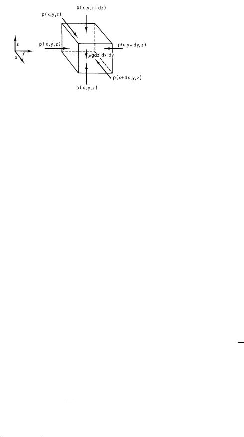
FIGURE 1.25. The fluid in volume dxdydz is in equilibrium.
only if p1 = p3, while the horizontal components sum to zero only if p3 = p2. Since this result is independent of the value of θ, the pressure must be the same in every direction.
Next, consider how the pressure changes with position. Suppose that p depends on the coordinates p = p(x, y, z) and that the density of the fluid is ρ kg m−3. The only external force acting is gravity in the direction of the −z axis. The fluid in the volume dxdydz of Fig. 1.25 is in equilibrium. In the y direction there is a force to the right across the left-hand face equal to p(x, y, z)dxdz and to the left across the right-hand face equal to −p(x, y +dy, z)dxdz. These are the only forces in the y direction, and their magnitudes must be the same. Therefore p does not change in the y direction. A similar argument shows that p does not change in the x direction. In the z direction there are three terms: the upward force across the bottom face, the downward force across the top face, and the pull of gravity. The weight of the fluid is its mass (ρ dxdydz) times the gravitational acceleration g (g = 9.8 m s−2). The three forces must add to zero:
p(x, y, z) dxdy − p(x, y, z + dz) dxdy − ρg dxdydz = 0.
For small changes in height, dz, it is possible to approximate7 p(x, y, z + dz) by p(x, y, z) + (dp/dz) dz. With this approximation, the equilibrium equation is
|
|
dp |
|
|
dxdydz |
− |
− ρg = 0. |
||
|
||||
dz |
This equation can be satisfied only if
dp |
= −ρg. |
(1.29) |
dz |
This is a di erential equation for p(z). It is a particularly simple one, since the right-hand side is constant if ρ and
7See Appendix D on Taylor’s series for a more complete discussion of this approximation.
g are constant: dp = −ρgdz. Integrating this gives
dp = −ρg dz,
p = −ρgz + c.
The constant of integration is determined by knowing the value of p for some value of z. If p = p0 when z = 0, then p0 = c and
p = p0 − ρgz. |
(1.30) |
With a constant gravitational force per unit volume acting on the fluid, the pressure decreases linearly with increasing height. The SI unit of pressure is N m−2 or pascal (Pa). The density is expressed in kg m−3, so that ρg has units of N m−3 and ρgz is in N m−2. Pressures are often given as equivalent values of z in some substance, for example, in millimeters of mercury (torr) or centimeters of water. In such cases, the value of z must be converted to an equivalent value of ρgz before calculations involving anything besides pressure are done. The density of water is 1 g cm−3 or 103 kg m−3. The density of mercury is 13.6 × 10³ kg m−3, so 1 torr = 133 Pa. Another common unit for pressure is the atmosphere (atm), equal to 1.01 × 10⁵ Pa. One atmosphere is approximately the atmospheric pressure at sea level.
1.12 Buoyancy
Buoyancy e ects are important when an object is immersed in a fluid. We are all familiar with buoyant e ects when swimming; they are also important in instruments such as the centrifuge. Consider an object of density ρ immersed in a fluid of density ρfluid. The net force on such an object is the sum of the gravitational force and a force arising from the pressure gradient in the fluid. To visualize this, consider a small object with sides dx, dy, dz. We have just seen that the pressure on the bottom face is greater than the pressure on the top face. Therefore there is an upward force on the cube. The total force on the object is then
dp |
− ρg dx dy dz. |
F = −dz |
Since the pressure gradient in the fluid is −ρfluidg, the total force is
F = (ρfluid − ρ) gV, |
(1.31) |
where V is the volume of the object. The second term is the object’s weight, directed downward. The first term is called the buoyant force and is directed upward. The buoyant force reduces the “e ective weight” of the object and depends on the di erence of densities of the object and the surrounding fluid.
Animals are made up primarily of water, so their density is approximately 103 kg m−3. The buoyant force depends on the animal’s environment. Terrestrial animals

live in air, which has a density of 1.2 kg m−3. The buoyant force on terrestrial animals is very small compared to their weight. Aquatic animals live in water, and their density is almost the same as the surrounding fluid. The buoyant force almost cancels the weight, so the animal is essentially “weightless.” Gravity plays a major role in the life of terrestrial animals, but only a minor role for aquatic animals. Denny (1993) explores the di erences between terrestrial and aquatic animals in more detail.
1.13 Compressibility
Increasing the pressure on a fluid causes a deformation and a decrease in volume. The compressibility κ is defined as
∆V |
= −κ∆p. |
(1.32) |
V |
Since ∆V /V is dimensionless, κ has the units of inverse pressure, N−1 m2 or Pa−1. In many liquids the compressibility is quite small (e.g., 5 ×10⁻¹⁰ Pa−1 for water), and for many purposes, such as flow through pipes, compressibility can be ignored. Other e ects, such as the transmission of sound through a fluid, depend on deformation, and compressibility cannot be ignored.
1.14 Viscosity
A fluid at rest does not support a shear. If the fluid is moving, a shear force can exist. At large velocities the flow of the fluid is turbulent and may be di cult or impossible to calculate. We will consider only cases in which the velocity is low enough so that the flow is smooth. This means that particles of dye introduced into the fluid to monitor its motion flow along smooth lines called streamlines. A streamline is tangent to the velocity vector of the fluid at every point along its path. There is no mixing of fluid across streamlines; the flow is laminar (in layers). Laminar flow is often used in rooms where dirt or bacterial contamination is to be avoided, such as operating rooms or manufacturing clean rooms. Clean air enters and passes through the room without mixing. Any contaminants picked up are carried out in the air.
A fluid can support a viscous shear stress if the shear strain is changing. One way to create such a situation is to immerse two parallel plates, each of area S, in the fluid, and to move one parallel to the other as in Fig. 1.26. If the fluid in contact with each plate sticks to the plate,8 the fluid in contact with the lower plate is at rest and that in contact with the upper plate moves with the same velocity as the plate. Between the plates the fluid flows parallel to the plates, with a speed that depends
8This is called the “no-slip” boundary condition. There are exceptions.
1.13 Compressibility |
15 |
v x = v
F
y
F
x
v x = 0
FIGURE 1.26. Forces F and −F are needed to make the top plate move in a viscous fluid while the bottom plate remains stationary. The velocity profile is also shown.
on position as shown in Fig. 1.26. The variation of velocity between the plates gives rise to a velocity gradient dvx/dy. Note that this is the rate of change of the shear strain.
In order to keep the top plate moving and the bottom plate stationary, it is necessary to exert a force of magnitude F on each plate: to the right on the upper plate and to the left on the lower plate. The resulting shear stress or force per unit area is in many cases proportional to the velocity gradient:
F |
= η |
dvx |
. |
(1.33) |
S |
|
|||
|
dy |
|
||
The constant η is called the coe cient of viscosity. Often this equation is written with a minus sign, in which case F is the force of the fluid on the plate rather than the plate on the fluid. The units of η are N s m−2 or kg m−1 s−1 or Pa s. Older units are the dyn s cm−2 or poise, the centipoise, and the micropoise. 1 poise = 0.1 Pa s. Equation 1.33 gives the force exerted by fluid above the plane at height y on the fluid below the plane. In the case of the parallel plates, the force from above on fluid in the slab between y and y + dy is the same in magnitude as (and opposite in direction to) the force exerted by the fluid below the slab. Therefore there is no net force on the fluid in the slab, and the fluid moves with constant velocity. Fluids that are described by Eq. 1.33 are called Newtonian fluids. Many fluids are not Newtonian.
Since dvx/dy is the rate of change of the shear strain, Eq. 1.27, Eq. 1.33 can be written
ss = FS = η ddts .
The rate of change of the shear strain is also called the shear rate.
1.15 Viscous Flow in a Tube
Biological fluid dynamics is a well-developed area of study [Lighthill (1975); Mazumdar (1992); Vogel (1994)]. External biological fluid dynamics is concerned with locomotion—from single-celled organisms to swimming
16 1. Mechanics
Rp |
2πr ∆x η dv / dr |
|
r
p(x )π r 2 |
p(x + ∆ x )πr 2 |
v |
|
End View |
Side View |
VelocityProfile |
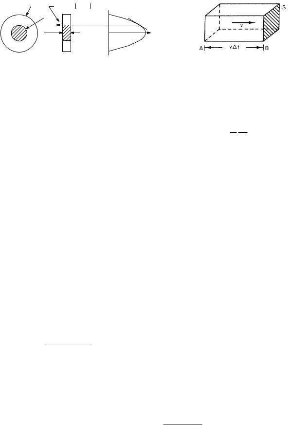
FIGURE 1.28. Flow of fluid across the plane at B. |
|
|
|
FIGURE 1.27. Longitudinal and transverse cross sections of the tube. Newton’s first law is applied to the shaded volume.
fish and flying birds. Internal biological fluid dynamics deals with mass transport within the organism. Two obvious examples are flow in the airways and the flow of blood.
Consider laminar viscous flow of fluid through a pipe of constant radius Rp and length ∆x. Ignore for now the gravitational force. The pressure at the left end of a segment of pipe is p(x); at the right end it is p(x + ∆x). For now consider the special case in which none of the fluid is accelerated, so the total force on any volume element of the fluid is zero. The velocity profile must be as shown in Fig. 1.27: zero at the walls and a maximum at the center. Our problem is to determine v(r).
Let us determine the forces acting on the shaded cylinder of fluid of radius r shown in Fig. 1.27. Since gravity is ignored, there are only three forces acting on the volume. The fluid on the left exerts a force πr2p(x) acting to the right in the direction of the positive x axis. The fluid on the right exerts a force −πr2p(x + ∆x) (the minus sign because it points to the left). The slower-moving fluid outside the shaded region exerts a viscous drag force across the cylindrical surface at radius r. The area of the surface is 2πr∆x. The force points to the left. Its magnitude is 2πr∆x η |dv/dr|. Since dv/dr is negative, we obtain the correct sign by writing it as 2πr ∆x η (dv/dr). Since the fluid is not accelerating, the forces sum to zero:
πr2 [p(x) − p(x + ∆x)] + 2πr ∆x η (dv/dr) = 0, (1.34)
which can be rearranged to give
dv |
= |
|
r |
|
p(x + ∆x) − p(x) |
|
||||||||||
|
|
|
|
|||||||||||||
|
dr |
2η |
||||||||||||||
|
|
|
|
∆x |
|
|
|
|
|
|
||||||
This can be integrated: |
|
|
|
|
|
|
|
|
|
|
||||||
|
|
|
|
|
dv = |
|
1 |
|
|
dp |
|
|||||
|
|
|
|
|
2η |
|
|
|||||||||
|
|
|
|
|
|
|
|
dx |
||||||||
|
|
|
|
|
v(r) = |
1 |
|
dp |
r2 |
|||||||
|
|
|
|
|
|
|
||||||||||
|
|
|
|
|
|
|
4η |
dx |
||||||||
= |
dp |
|
r |
. |
(1.35) |
|
|
||||
dx 2η |
|
||||
r dr,
+ A. |
(1.36) |
For flow to the right dp/dx is negative. Therefore it is convenient to write ∆p as the pressure drop from x to x+ dx: ∆p = p(x)−p(x+∆x). Then the first term in Eq. 1.36 is −(1/4η)(∆p/∆x)r2. The constant of integration can be
determined assuming the “no-slip” boundary condition: that the velocity of the fluid immediately adjacent to a solid is the same as the velocity of the solid itself. Because the wall is at rest, the velocity of the fluid is zero at the wall (r = Rp). The final result is
v(r) = |
1 ∆p |
(Rp2 − r2). |
(1.37) |
4η ∆x |
The total flow rate or volume flux or volume current i is the volume of fluid per second moving through a cross section of the tube. Its units are m3 s−1. The volume fluence rate or volume flux density9 or current density jv is the volume per unit area per unit time across some
small area in the tube. The units of jv are m3 s−1 m−2 or m s−1.
In fact, jv is just the velocity of the fluid at that point. To see this, consider the flow of an incompressible fluid during time ∆t. In Fig. 1.28 the fluid moves to the right with velocity v. At t = 0, the fluid just to the left of plane B crosses the plane; at t = ∆t, that fluid that was at A at t = 0 crosses plane B. All the fluid between plane A and plane B crosses plane B during the time interval ∆t. The volume fluence rate is
jv = |
(volume transported) |
= |
Sv∆t |
= v. |
(1.38) |
|
(area)(time) |
|
S∆t |
||||
It may seem unnecessarily confusing to call the fluence rate or flux density jv instead of v; however, this notation corresponds to a more general notation in which j means the fluence rate or flux density of anything per unit area per unit time, and the subscript v, s, or q tells us whether it is the fluence rate of volume, solute particles, or electric charge.
To find the volume current i, jv must be integrated over the cross-sectional area of the pipe. The volume of fluid crossing the washer-shaped area 2πrdr is jv 2πrdr = v2πrdr. The total flux through the tube is therefore
Rp
i = jv (r)2πr dr,
|
0 |
|
|
|
|
|
|||
i = |
2π ∆p Rp |
2 |
|
2 |
|
(1.39) |
|||
|
|
|
0 |
Rp |
− r |
|
r dr. |
||
4η |
∆x |
|
|||||||
9Some authors call jv the flux. The nomenclature used here is consistent throughout the book.

To integrate this, let u = Rp2 − r2. Then du = −2rdr and the integral is Rp4/4. Therefore
πRp4 ∆p |
(1.40) |
i = 8η ∆x |
is the flux of a viscous fluid through a pipe of radius Rp due to a pressure gradient (∆p/∆x) along the pipe. The dependence of i on Rp4 means that small changes in diameter cause large changes in flow.
This relationship was determined experimentally in painstaking detail by a French physician, Jean Leonard Marie Poiseuille, in 1835. He wanted to understand the flow of blood through capillaries. His work and knowledge of blood circulation at that time have been described by Herrick (1942).
As an example of the use of Eq. 1.40, consider a pore of the following size, which might be found in the basement membrane of the glomerulus of the kidney:
Rp = 5 nm, |
|
|
|
|
∆p = 15.4 torr, |
|
|
(1.41) |
|
η = 1.4 × 10⁻³ kg m−1 |
s−1 |
, |
||
|
∆x = 50 nm.
It is first necessary to convert 15.4 torr to Pa using Eq. 1.30 and the value of ρ for mercury, 13.55×10³ kg m−3:
∆p = ρg∆z = (13.55 × 10³)(9.8)(15.4 × 10⁻³) = 2.04 × 10³ N m−2.
Then Eq. 1.40 can be used:
i = (3.14)(5 × 10⁻⁹)4(2.04 × 10³) = 7.2 × 10⁻²¹ m3 s−1. (8)(1.4 × 10⁻³)(50 × 10−9)
Now consider the general case in which we have not only viscosity, but the fluid may be accelerated and gravity is important. We continue to write ∆p as the pressure drop and consider four contributions, each of which will be discussed:
x2
∆p = |
(dp/dx) dx |
(1.42) |
x1
= ∆pvisc + ∆pgrav + ∆paccel1 + ∆paccel2.
For simplicity, we restrict the derivation to an incompressible fluid and a pipe of circular cross section where the radius can change. The distance along the pipe is x and the radius of the pipe is Rp(x). Gravitational force acts on the fluid, and the height of the axis of the pipe above some reference plane is z, as shown in Fig. 1.29.
Because the fluid is incompressible, the total current i is independent of x. If the pipe narrows, the velocity increases. Assume that changes in pipe radius occur slowly enough so that the velocity profile remains parabolic at every point in the pipe and we can treat x as though it
1.15 Viscous Flow in a Tube |
17 |
FIGURE 1.29. A pipe of circular cross section with radius and height varying along the pipe.
were a distance along the axis of the cylinder. If we define the average velocity as
|
|
|
|
|
(x) = |
|
|
i |
|
, |
(1.43) |
||||
|
|
|
v |
|
|
|
|||||||||
|
|
|
πR2 |
(x) |
|||||||||||
|
|
|
|
|
|
|
|
|
p |
|
|
|
|
|
|
we can use Eq. 1.37 to rewrite the velocity profile as |
|||||||||||||||
v(r, x) = 2 |
|
1 − |
|
r2 |
= |
|
|
2i |
1 − |
r2 |
|||||
v |
|
|
|
|
|
. |
|||||||||
Rp2(x) |
πRp2(x) |
Rp2(x) |
|||||||||||||
|
|
|
|
|
|
|
|
|
|
|
|
|
(1.44) |
||
The first term in Eq. 1.42 is the pressure to overcome viscous drag. We can rewrite Eq. 1.35 as
|
|
dpvisc |
= |
|
2η |
|
dv |
. |
|
|
||
|
|
|
|
|
||||||||
|
|
dx |
|
|
|
r dr |
|
|||||
Using Eq. 1.44 we can write |
|
|
|
|
|
|
|
|||||
|
dpvisc |
= − |
|
8η i |
(1.45) |
|||||||
|
|
|
|
. |
||||||||
|
dx |
πRp4(x) |
||||||||||
We saw this earlier, solved for i in a pipe of constant radius, as Eq. 1.40. The pressure drop is obtained by integration:
|
x2 |
|
|
x2 |
dpvisc |
|
||
∆pvisc = − x1 |
dpvisc = − x1 |
|
|
dx (1.46) |
||||
|
dx |
|||||||
= + |
8ηi |
x2 |
dx |
. |
|
|
|
|
|
π |
x1 |
R4(x) |
|
|
|
||
|
|
|
p |
|
|
|
||
To go further requires knowing Rp(x).
The next term pgrav is the hydrostatic pressure change that we saw in Eq. 1.30:
x2 |
|
dpgrav |
dz = ρg(z2 − z1). |
|
∆pgrav = − x1 |
dpgrav = − |
|
|
|
|
dz |
|||
(1.47) The last two terms of Eq. 1.42 are pressure di erences required to accelerate the fluid. When the flow is steady— that is, the velocity depends only on position, and the
18 1. Mechanics
velocity at a fixed position does not change with time— there can still be an acceleration if the cross section of the pipe changes. The third term, ∆paccel1, provides the force for this acceleration. It can be derived as follows. Imagine a streamline in the fluid. No fluid crosses the streamline. Consider a small length of streamline ds and a small area dA perpendicular to it. Note that ds is a small displacement along a streamline, while dx is along the axis of the pipe. The edge of dA defines another set of streamlines that form a tube of flow, and dAds defines a small volume of fluid. Make ds and dA small enough so that v is nearly the same at all points within the volume. The mass of fluid in the volume is dm = ρdAds. We ignore viscosity and gravity, so the only pressure di erence is due to acceleration. The net force on the volume is
dp |
(1.48) |
dF = −ds ds dA. |
This is equal to the mass times the acceleration dv/dt. The acceleration of the fluid in the element is then
|
|
|
|
|
|
|
|
|
|
|
|
dv |
= |
dF |
= |
− dpds |
dsdA |
= − |
1 |
dp |
|
||
|
|
|
|
|
|
|
. (1.49) |
||||
dt |
dm |
|
ρdsdA |
ρ |
|
ds |
|||||
We are considering only velocity changes that occur because the fluid moves along a streamline to a di erent position. We use the chain rule to write
|
|
|
dv |
= |
|
dv |
|
ds |
|
= v |
dv |
. |
|
|
|
|
|||||||||
|
|
|
|
|
|
ds |
|
dt |
|
|
|
|
|
||||||||||||
|
|
|
dt |
|
|
|
|
|
|
ds |
|
|
|
|
|||||||||||
Combining these gives |
|
|
|
|
|
|
|
|
|
|
|
|
|
|
|||||||||||
|
|
|
|
|
|
dpaccel1 |
= |
−ρv |
dv |
|
|
|
|
|
(1.50) |
||||||||||
|
|
|
|
|
|
|
|
|
|
|
|
|
. |
|
|
|
|
|
|||||||
|
|
|
|
|
|
|
|
ds |
ds |
|
|
|
|
|
|||||||||||
This can be integrated along the streamline to give |
|||||||||||||||||||||||||
|
|
|
s2 |
dpaccel1 |
|
|
|
|
x2 |
|
dv |
|
|||||||||||||
∆paccel1 = − s1 |
|
|
|
|
|
|
|
ds = +ρ |
|
|
v |
|
|
ds |
|||||||||||
|
|
|
|
ds |
|
|
|
x1 |
|
ds |
|||||||||||||||
= |
ρv2 |
|
ρv2 |
|
|
|
|
|
|
|
|
|
|
|
|
|
(1.51) |
||||||||
|
|
2 |
− |
|
1 |
. |
|
|
|
|
|
|
|
|
|
|
|
|
|
||||||
|
|
2 |
2 |
|
|
|
|
|
|
|
|
|
|
|
|
|
|||||||||
The final term ∆paccel2 is the pressure change required to accelerate the fluid between points 1 and 2 if the velocity of the fluid at a fixed position is changing with time. This happens, for example, to blood that is accelerated as it is ejected from the heart during systole, or to fluid that is sloshing back and forth in a U tube. To derive this term, again imagine a small length of streamline ds and a small area dA perpendicular to it. In addition to ignoring gravity and viscosity, we ignore changes in velocity because of changes in cross section. There is acceleration only if the velocity at a fixed location is changing. The acceleration is ∂v/∂t. The derivative is written with ∂’s to signify the fact that we are considering only changes in the velocity with time that occur at a fixed position.
The net force required to accelerate this mass is provided by the pressure di erence Eq. 1.48:
|
|
∂v |
|
|
∂v |
|
||||
dF = −dA dpaccel2 = dm |
|
|
|
= ρ |
|
|
dA ds, |
|||
∂t |
∂t |
|||||||||
|
∂v |
|
|
|
|
|
||||
dpaccel2 = −ρ |
|
|
|
ds, |
|
|
|
|||
|
∂t |
|
|
|
||||||
s2 |
|
|
s2 |
∂v |
|
|||||
∆paccel2 = − s1 |
dpaccel2 = ρ |
|
|
|
|
ds. (1.52) |
||||
s1 |
|
∂t |
||||||||
All of these e ects can be summarized in the generalized Bernoulli equation:
|
|
|
|
|
|
|
|
s2 |
∂v |
|
|
|
|
s2 |
|
dpvisc |
|
|
||||||||||
p1 − p2 = ∆p = ρ |
|
|
|
|
|
|
|
|
ds + s1 |
− |
|
|
|
ds |
||||||||||||||
|
s1 |
|
∂t |
|
ds |
|||||||||||||||||||||||
|
|
|
|
|
|
|
|
|
|
|
|
|
|
|
|
|
|
|
|
|
|
|
|
|||||
|
|
|
|
|
|
|
|
|
|
accel2 |
|
|
|
∆ |
visc |
|
||||||||||||
|
|
|
|
|
|
|
|
|
∆p |
|
|
|
|
|
|
|
|
|
|
|
|
p |
|
|
||||
|
|
|
|
|
|
|
|
|
|
|
|
|
|
|
|
|
|
|
|
|
|
|
|
|
|
|
(1.53) |
|
+ |
ρv2 |
ρv2 |
|
|
|
|
|
|
|
|
|
|
|
|
|
|
|
|
|
|||||||||
2 |
− |
1 |
+ ρg (z |
2 − z1 |
) |
|
|
|
|
|
|
|||||||||||||||||
2 |
|
2 |
|
|
|
|
|
|
|
|||||||||||||||||||
|
|
|
|
|
|
|
|
|
|
|
|
|
|
∆ |
|
|
|
|
|
|
|
|
|
|
|
|||
|
|
∆paccel1 |
|
|
|
|
|
|
|
p |
|
|
|
|
|
|
|
|
|
|||||||||
|
|
|
|
|
|
|
|
grav |
|
|
|
|
|
|
|
|
|
|||||||||||
Equation 1.53 is valid for nonuniform viscous flow that may be laminar or turbulent if the integral is taken along a streamline [see, for example, Synolakis and Badeer (1989)].
1.16 Pressure–Volume Work
An important example of work is that done in a biological system when the volume of a container (such as the lungs or the heart or a blood vessel) changes while the fluid within the container is exerting a force on the walls.
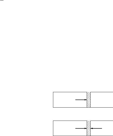
To deduce an expression for pressure–volume work, consider a cylinder of gas fitted with a piston, Fig. 1.30(a). If the piston has area S, the gas exerts a force Fg = pS on the piston. If no other force is exerted on the
S
Fg
(a)
Fg Fe
(b)
FIGURE 1.30. (a) A cylinder containing gas has a piston of area S at one end. (b) The force exerted on the piston by the gas is balanced by an external force if the piston is at rest.
1.17 The Human Circulatory System |
19 |
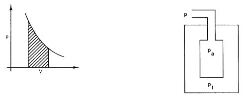
FIGURE 1.31. A plot of p vs V , showing the work done by the gas as it expands.
piston to restrain it, it will be accelerated to the right and gain kinetic energy as the gas does work on it:
FIGURE 1.32. A model of the thorax, lungs, and airways that can be used to understand some features of breathing.
(work done by gas) = Fg dx = pSdx = pdV. (1.54)
If the piston is prevented from accelerating by an external force Fe equal and opposite to that exerted by the gas [Fig. 1.28(b)], then the external force does work on the piston:
(work done by external force) = −Fedx |
(1.55) |
= −pSdx = −pdV,
which is the negative of the work done on the piston by the expanding gas. The result is that the kinetic energy of the piston does not change. The gas does work on the surroundings as it expands, increasing the energy of the surroundings; the surroundings, through the external force, do negative work on the gas; that is, they decrease the energy of the gas. (The meaning of “energy of the gas” and “energy of the surroundings” is discussed in Chapter 3.) If the gas is compressed, the situation is reversed: the surroundings do positive work on the gas and the gas does negative work on the surroundings.
For a large change in volume from V1 to V2, the pressure may change as the volume changes. In that case the work done by the gas on the surroundings is
V2
Wby gas = |
p dV. |
(1.56) |
V1
This work is the shaded area in Fig. 1.31. If the gas is compressed, the change in volume is negative and the work done by the gas is negative.
Let us apply this model to the heart. Suppose that the left ventricle of the heart contracts at constant pressure, so that it changes volume by ∆V = V2 − V1. (Since V2 < V1 the quantity ∆V is negative. A volume of blood −∆V is ejected into the aorta.) The work done by the heart wall on the blood is −p∆V and is positive, since ∆V is negative.
As another example of pressure–volume work, we can develop a model to estimate the work necessary to breathe. Consider the model of the lungs and airways shown in Fig. 1.32. The pressure at the nose is the atmospheric pressure p. In the alveoli (air sacs) the pressure
is pa. If there is no flow taking place, pa = p. For air to flow in, pa must be less than p; for it to flow out, pa must be greater than atmospheric. The work done by the walls
of the alveoli on the gas in them is − pa dV . The net value of this integral for a respiratory cycle is positive. Perhaps the easiest way to see this is to imagine an inspiration, in which the alveolar pressure is pa = p − ∆p and the volume change is ∆V . The work done on the gas is −(p − ∆p)∆V . This is followed by an expiration at pressure pa = p + δp, for which the work is −(p + δp)(∆V ). The net work done on the gas is (∆p+δp)∆V . The energy imparted to the gas shows up as a mixture of heating because of frictional losses and kinetic energy of the exhaled air.
There is another mechanism by which work is done in breathing. Refer again to Fig. 1.32. The pressure in the chest cavity (thorax) is pt. (The pressure measured in mid-esophagus is a good estimate of pt.) Because of contractile forces in the lung tissue, pa > pt. The quantity pa − pt is the “elastic recoil pressure” of Fig. 1.22. The gas in the alveoli and the fluid in the thorax both do work on the lung tissue. The latter has opposite sign, since a positive displacement dx of a portion of the alveolar wall is in the direction of the force exerted by the alveolar gas but is opposite to the direction of the force exerted by the thoracic fluid. The elastic recoil pressure, multiplied by dV , gives the net work done by both forces on the wall of the lung.
Figure 1.22 shows elastic recoil pressure versus lung volume. It is redrawn in Fig. 1.33. During inspiration (curve AB), the elastic recoil pressure pa − pt is greater than that during expiration (curve BC). The net work done on the lung wall during the respiratory cycle goes into frictional heating of the lung tissue.
1.17 The Human Circulatory System
The human circulatory system is responsible for pumping blood and its life-sustaining nutrients to all parts of
20 1. Mechanics
FIGURE 1.33. A hypothetical plot of the pressure–volume relationship for inhalation and exhalation.
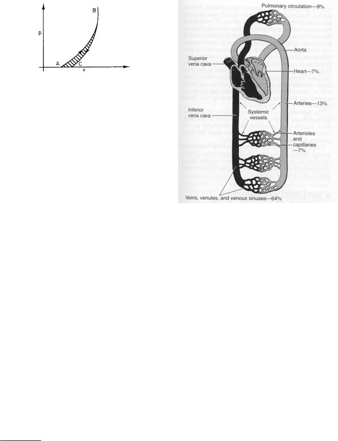
the body [Vogel (1992)]. The circulatory system has two parts: the systemic circulation and the pulmonary circulation, as shown in Fig. 1.34. The left heart pumps blood into the systemic circulation: organs, muscles, etc. The right heart pumps blood through the lungs. As the heart beats, the pressure in the blood leaving the heart rises and falls. The maximum pressure during the cardiac cycle is the systolic pressure. The minimum is the diastolic pressure. (A blood pressure reading is in the form systolic/diastolic, measured in torr.) The blood flows from the aorta to several large arteries, to medium-sized arteries, to small arteries, to arterioles, and finally to the capillaries, where exchange with the tissues of oxygen, carbon dioxide, and nutrients takes place. The blood emerging from the capillaries is collected by venules, flows into increasingly larger veins, and finally returns to the heart through the vena cava.
At any given time, blood is flowing in only a fraction of the capillaries. The state of flow in the capillaries is continually changing to provide the amount of oxygen required by each organ. In skeletal muscle, terminal arterioles constrict and dilate to control distribution of blood to groups of capillaries. In smooth muscle and skin, a precapillary sphincter muscle controls the flow to each capillary [Patton et al. (1989), p. 860]. Since the blood is incompressible and is conserved,10 the total volume flow i remains the same at all generations of branching in the vascular tree. Table 1.4 shows average values for the pressure and vessel sizes at di erent generations of branching. Most of the pressure drop occurs in the arterioles.
We define the vascular resistance R in a pipe or a segment of the circulatory system as the ratio of pressure di erence across the pipe or segment to the flow through it:
R = |
∆p |
. |
(1.57) |
|
|||
|
i |
|
|
The units are Pa m−3 s. Physiologists use the peripheral resistance unit (PRU), which is torr ml−1 min. For Poiseuille flow the resistance can be calculated
10This is not strictly true. Some fluid leaves the capillaries and returns to the heart through the lymphatic system instead of the venous system. See Chapter 5.
FIGURE 1.34. The human circulatory system. The subject is facing you, so the left chambers of the heart are on the right in the picture. The left heart pumps oxygenated blood (gray), and the right heart pumps deoxygenated blood (black). Reprinted from A.C. Guyton. Textbook of Medical Physiology, 8th ed. p. 151. c 1991 Elsevier, Inc. Used with permission of Elsevier.
from Eq. 1.40:
R = |
8η∆x |
. |
(1.58) |
|
The resistance decreases rapidly as the radius of the vessel increases.
If vessels of di erent diameters are connected in series so that the flow i is the same through each one and the total pressure drop is the sum of the drops across each vessel, then the total resistance is the sum of the resistances of each vessel:
Rtot = R1 + R2 + R3 + · · · . |
(1.59) |
If there is branching so that several vessels are in parallel with the same pressure drop across each one, the total flow through all the branches equals the flow in the vessel feeding them. The total resistance is then given by
1 |
= |
|
1 |
+ |
1 |
+ |
|
1 |
+ · · · . |
(1.60) |
Rtot |
R1 |
R2 |
R3 |
|||||||
For the most part, the capillaries are arranged in parallel. Even though the resistance of an individual capillary is large because of its small radius (Eq. 1.58), the resistance

1.18 Turbulent Flow and the Reynolds Number |
21 |
TABLE 1.4. Typical values for the average pressure at the entrance to each generation of the major branches of the cardiovascular tree, the average blood volume in certain branches, and typical dimensions of the vessels.
Location |
Average |
Blood |
Diameterb |
Lengthb |
Wall |
Avg. |
Reynolds number at |
|
pressure |
volumea |
(mm) |
(mm) |
thicknessb |
velocityb |
maximum flow c |
|
(torr) |
(ml) |
|
|
(mm) |
(m s−1) |
|
Left atrium |
5 |
|
Systemic circulation |
|
|
|
|
|
|
|
|
|
|
||
Left ventricle |
100 |
|
|
|
|
4.80×10⁻¹ |
9 400 |
Aorta |
100 |
156 |
20 |
500 |
2.00 |
||
Arteries |
95 |
608 |
4 |
500 |
1.00 |
4.50×10⁻¹ |
1 300 |
Arterioles |
86 |
94 |
0.05 |
10 |
0.2 |
5.00×10⁻² |
|
Capillaries |
30 |
260 |
0.008 |
1 |
0.001 |
1.00×10⁻³ |
|
Venules |
10 |
470 |
0.02 |
2 |
0.002 |
2.00×10⁻³ |
|
Veins |
4 |
2682 |
5 |
25 |
0.5 |
1.00×10⁻² |
|
Vena cava |
3 |
125 |
30 |
500 |
1.5 |
3.80×10⁻¹ |
3 000 |
Right atrium |
3 |
|
Pulmonary Circulation |
|
|
|
|
Right atrium |
3 |
|
|
|
|
||
|
|
|
|
|
|
||
Right ventricle |
25 |
|
|
|
|
|
|
Pulmonary artery |
25 |
52 |
|
|
|
|
|
Arteries |
20 |
91 |
|
|
|
|
7 800 |
Arterioles |
15 |
6 |
|
|
|
|
|
Capillaries |
10 |
104 |
|
|
|
|
|
Veins |
5 |
215 |
|
|
|
|
2 200 |
Left atrium |
5 |
|
|
|
|
|
|
|
|
|
|
|
|
|
|
aFrom R. Plonsey (1995). Physiologic Systems. In J. R. Bronzino, ed. The Biomedical Engineering Handbook, Boca Raton, CRC Press, pp. 9–10.
bFrom J. N. Mazumdar (1992). Biofluid Mechanics. Singapore, World Scientific, p. 38.
cFrom W. R. Milnor (1989). Hemodynamics, 2nd. ed. Baltimore, Williams & Wilkins, p. 148.
of the capillaries as a whole is relatively small because there are so many of them (see Problem 41).
The average flow from the heart is the stroke volume— the volume of blood ejected in each beat—multiplied by the number of beats per second. A typical value might be
i = (60 ml beat−1)(80 beat min−1) = 4800 ml min−1 = 80 × 10−6 m3 s−1.
The total resistance would then be the average pressure divided by the flow:
R = (100 torr)(133 Pa torr−1) = 1.66 × 10⁸ Pa m−3 s. 80 × 10−6 m3 s−1
nearly constant volume that causes the ventricular pressure to rise until it exceeds the (diastolic) pressure in the aorta, and the aortic valve opens. The contraction continues, and the pressure rises further, but the ventricular volume decreases as blood flows into the aorta. The ventricle then relaxes. The aortic valve closes when the ventricular pressure drops below that in the aorta. The work done in one cycle is the area enclosed by the curve. For the curve shown, it is 6600 torr ml = 0.88 J. At 80 beats per minute the power is 1.2 W. In this drawing the stroke volume is 100−35 = 65 ml, and the cardiac output is
i = (65 ml beat−1)(80 beats/60 s) = 87 × 106m3s−1.
The pressure in the left ventricle changes during the cardiac cycle. It can be plotted vs time. It can also be plotted vs ventricular volume, as in Fig. 1.35. The p– V relationship moves counterclockwise around the curve during the cycle. Filling occurs at nearly zero pressure until the ventricle begins to distend when the volume exceeds 60 ml. There is then a period of contraction at
1.18Turbulent Flow and the Reynolds Number
Many features of the circulation can be modeled by Poiseuille flow. However, at least four e ects—in addition to those in Eq. 1.42—cause departures from Poiseuille