Intermediate Physics for Medicine and Biology - Russell K. Hobbie & Bradley J. Roth

4.1.6The Continuity Equation with a Chemical Reaction

Our derivation of the continuity equation assumed that the substance was conserved—neither created nor destroyed. If a chemical reaction is creating the substance at a rate Q particles m−3 s−1 (which may depend on position) then the continuity equation becomes

the volume

If particles are being consumed in the chemical reaction, then Q is negative.

4.2 Drift or Solvent Drag

One simple way that solute particles can move is to drift with constant velocity. They can do this in a uniform electric or gravitational field if they are also subject to viscous drag, or they can be carried along by the solvent, a process called drift or solvent drag. (The solute particles are dragged by the solvent.) The solute fluence rate is js, with units of particles m−2 s−1 or just m−2 s−1. The number of solute particles passing through a surface is the volume of solution that moves through the surface times the concentration of solute particles. Therefore,

This e ect will be explored in greater detail in Sec. 4.12.

4.3 Brownian Motion

There is also movement of solute molecules when the water is at rest. If the solution is dilute, the solute particles are far apart and hit one another only occasionally. They are struck by water molecules much more often. The result is that they are in continual helter-skelter motion. Each solute molecule is influenced by water molecules, but not by other solute molecules.

In Chapter 3, it was shown that the relative probability for a particle to have energy u when it is in thermal equilibrium with a reservoir at temperature T is given by a Boltzmann factor:3P e−u/kB T . In Chapter 3, the

3The Boltzmann factor provided Jean Perrin with the first means to determine Avogadro’s number. The density of particles

TABLE 4.2. Values of the rms velocity for various particles at body temperature.

Boltzmann factor was used to show that if any energy term depends on the square of some variable, then the average value of that term is kB T /2. A particle with kinetic energy of translation m(vx2 + vy2 + vz2)/2 has an average energy kB T /2 for each of the three terms, or a total translational kinetic energy of 3kB T /2. This is true regardless of the mass of the particle. Any particle in thermal equilibrium with a reservoir (which can be the surrounding fluid) will move with a mean square velocity given by4

The square root of v2 is called the root-mean-square, or rms, velocity. It decreases with increasing mass of the

particle. Table 4.2 shows values of vrms = (v2)1/2 for different particles at body temperature.

This movement of microscopic-sized particles, resulting from bombardment by much smaller invisible atoms, was first observed by the English botanist Robert Brown in 1827 and is called Brownian motion. Solute particles are also subject to this random motion. If the concentration of particles is not uniform, there will be more particles wandering from a region of high concentration to one of low concentration than vice versa. This motion is called di usion.

In the next several sections, we study random motion and di usion, first for a gas and then for a liquid.

4.4Motion in a Gas: Mean Free Path and Collision Time

It is possible to define a mean free path, which is the average distance a particle travels between successive

in the atmosphere is proportional to exp(−mgy/kB T ), where mgy is the gravitational potential energy of the particles. Using particles for which m was known, Perrin was able to determine kB for the first time. Since the gas constant R was already known, Avogadro’s number was determined from the relationship R = NAkB .

4The average velocity is v¯x = 0, since a particle with a given speed moves with equal probability to the left or right.

86 4. Transport in an Infinite Medium

collisions, and a collision time, the average length of time between collisions. Consider a collection of N0 molecules. The number that have moved distance x without su ering a collision is N (x). For short distances dx, the probability that a molecule collides with another molecule is proportional to dx: call it (1/λ)dx. Then, on the average, the number of molecules having their first collision between x and x + dx is dN = −N (x)(1/λ)dx. This is the familiar equation for exponential decay. The number of molecules surviving without any collision is N (x) = N0e−x/λ.

To compute the average distance traveled by a molecule between collisions, we multiply each possible value of x by the number of molecules that su er their first collision between x and x+dx. Since N (x) is the number surviving at distance x, and dx/λ is the probability that one of those will have a collision between x and x + dx, the mean value of x is

With the substitutions s = x/λ and N (x) = N0e−s, this can be written as

∞

x = λ e−ss ds (4.13)

0

= −λ e−s(s + 1) ∞0 = λ.

Thus λ is the mean free path.

A similar argument can be made for the length of time that each molecule survives before being hit. The probability that a molecule is hit during a short time dt is proportional to dt: call it (1/tc)dt. The number of molecules surviving a time t is given by N = N0e−t/tc , and the mean time between collisions can be calculated as above. It is tc, which is called the collision time. The number of collisions per second is the collision frequency, 1/tc.

It is possible to estimate the mean free path and the collision frequency. Consider a particle of radius a1 moving through a dilute gas of other particles of radius a2. For convenience, imagine that particle 1 is moving and that all the other particles are fixed in position. The path of the first particle is shown in Fig. 4.6. If the center of one of these other molecules lies within a distance a1 + a2 of the

moving molecule, there will be a collision. The e ect is the same as if the moving particle had radius a1 + a2 and all the other particles were points. In moving a distance x, the particle sweeps out a volume V (x) = π(a1 + a2)2x. On average, when the particle has traveled a mean free path there is one collision. The average number of gas particles in the volume V (λ) = π(a1 + a2)2λ is therefore 1. The average number of particles per unit volume is C. Thus, 1 = Cπ(a1 + a2)2λ, or

The quantity π(a1 +a2)2 is the area of a circle. It is called the cross section for the collision of these particles. The concept of cross section is used extensively in Chapter 15.

This estimation is somewhat crude in its assumption that only one molecule is moving. If all the molecules are of the same kind, then the factor 1 in the numerator is replaced by 2−1/2 = 0.707 [Reif (1965, p. 471)].

For a gas at standard temperature and pressure, the volume of 1 mol is 22.4 liter = 22.4 × 10−3 m3, so C = 2.7 × 1025 m−3. If a1 = a2 = 0.15 nm, then Eq. 4.14 can be used to calculate the mean free path:

1

λ = (3.14)(.3 × 10−9)2 m2(2.7 × 1025 m−3)

= 0.13 µm.

For a gas at standard temperature and pressure, the mean free path is about 1000 times the molecular diameter, and the assumption of infrequent collisions is justified.

The collision time can be estimated by saying that

λ

tc = v ,

where v is the average speed of the molecules. Using the rms velocity for v, we can use Eq. 4.12 to write

The important feature of this is the dependence on m1/2 and on λ. For air at room temperature, tc = 2 × 10−10 s.

FIGURE 4.6. A particle of radius a1 moves through a gas of particles of radius a2. A collision will occur if the center of another particle lies within a distance a1 +a2 of the trajectory of the particle under consideration.

4.5 Motion in a Liquid

The assumptions of the previous section do not hold in a liquid, in which the particle is being continually bombarded by neighbors. Blindly applying Eq. 4.14 to water, we can use the fact that 1 mol is 18 g and occupies 18 cm3, to obtain λ = 0.1 nm, so that a/λ ≈ 1, and the assumptions behind the derivation break down. Estimating the collision time with Eq. 4.15 gives a value that is a factor of 1000 less than for the gas, or 10−13 s.

Although these estimates of the mean free path and the collision time are undoubtedly wrong, the concepts

appear to be valid. Computer simulations of molecular collisions show that the distribution of free paths is exponential even though the mean free path is only a fraction of a molecular diameter. In Sec. 4.12 we will regard di u- sion as a random walk of the di using particles and relate the di usion constant to the mean free path and collision time. Equations 4.14 and 4.15 can then be used to show that the di usion constant should be inversely proportional to the square of the particle radius. This has been verified experimentally for the di usion of certain liquids. Evidence for the validity of this random-walk model for di usion in liquids has been summarized by Hildebrand et al. (1970, pp. 36–39).

A particle in a liquid is subject to a fluctuating force F(t), which is random in magnitude and direction. The particle begins to move in response to this force. However, after it has begun to move, it su ers more collisions in front than behind, so the force slows it down. Because the particle can neither stay at rest nor continue to move in the same direction, it undergoes a random, zig-zag motion with average translational kinetic energy 3kB T /2. The mean square velocity is not zero, but the mean vector velocity is zero.

For each particle, Newton’s second law is m(dv/dt) = F(t). This is not very useful as it stands. To make it more tractable, consider a particle with average velocity v. (The average means that an ensemble of identically prepared particles is examined.) The particle has more collisions on the front that slow it down. We therefore break up F(t) into two parts: an average drag force, which will be the same for all the particles in the ensemble, and a rapidly fluctuating part g(t), which will vary with time and from particle to particle. Newton’s second law is then m(dv/dt) = (drag force) + g(t), where g(t) is random in direction. The drag force will be zero when v is zero. For average velocities that are not too large it can be approximated by a linear term:

(drag force) = −β v.

With this approximation, Newton’s second law is known as the Langevin equation:

(If the liquid is moving, the drag force will be zero when the particle has the same average velocity as the liquid. So v can be interpreted as the relative velocity of the particle with respect to the liquid.) This equation often has another term in it, which does not average to zero and which represents some external force such as gravity that acts on all the particles. This approximate equation can be solved in some cases, though with di culty, and has formed the basis for some treatments of the motion of large particles in fluids. With suitable interpretation, it can describe motion of the fluid molecules themselves.5

5See, for example, Pryde (1966, p. 161).

In particular, when dealing with molecular motion it is necessary to consider the fact that the molecules do not move independently of one another.

For a Newtonian fluid (Eq. 1.33) with viscosity η, one can show (although it requires some detailed calculation6) that the drag force on a spherical particle of radius a is given by

This equation is valid when the sphere is so large that there are many collisions of fluid molecules with it and when the velocity is low enough so that there is no turbulence. This result is called Stokes’ law.

If the sphere is not moving in an infinite medium but is confined within a cylinder, then a correction must be applied.7 In that case the viscous drag depends on the velocity of the spherical particle through the fluid, the average velocity of the fluid through the cylinder, and the distance of the particle from the axis of the cylinder.8

4.6 Di usion: Fick’s First Law

Di usion is the random movement of particles from a region of higher concentration to a region of lower concentration. The di using particles move independently of one another; they may collide frequently with the molecules of the fluid in which they are immersed, but they rarely collide with one another. The surrounding fluid may be at rest, in which case di usion is the only mechanism for transport of the solute, or it may be flowing, in which case it carries the solute along with it (solvent drag). Both e ects can occur together.

We first consider di usion from a macroscopic point of view and write down an approximate di erential equation to describe it. We then obtain a second equation describing di usion by combining this with the continuity equation. After discussing some solutions to these

6This is an approximate equation. See Barr (1931, p. 171).

7An early correction for particles on the axis of a cylinder is found in Barr (1931), p. 183. More recent work is by Levitt (1975), Bean (1972), and Paine and Scherr (1975).

8Stokes’ law is valid for a particle in a gas if the mean free path is much less than the particle radius a, so that many collisions with neighboring molecules occur. At the other extreme, a mean free path much greater than the particle radius, the drag force turns out to be Fdrag = αηa(a/λ)v. Although this will not be directly useful to us in considering biological systems, it is mentioned here to show how important it is to understand the conditions under which an equation is valid. Although the dimensions of this new equation are unchanged (we have introduced a factor a/λ, which is dimensionless), the drag force depends on a2 instead of on a. The reason for the di erence is that collisions are now infrequent and that the probability of a collision that imparts some average momentum change is proportional to the projected cross-sectional area of the sphere, πa2. In the regime of interest to us, in which there are many collisions, we would not expect the force to depend on λ. We hope that this will convince you of the danger in using someone else’s equation without understanding it.

Constant D is called the di usion constant. The units of D are m2 s−1, as may be seen by noting that the units of j are (something) m−2 s−1 and the units of ∂C/∂x are (something) m−4. This relationship is called Fick’s first law of di usion, after Adolf Fick, a German physiologist in the last half of the nineteenth century. The minus sign shows that the flow is in the direction from higher concentration to lower concentration: if ∂C/∂x is positive, the flow is in the −x direction.

If the actual process is not linear, this can be thought of as the first term of a Taylor’s series expansion (Appendix D).

Fick’s first law is one of many forms of the transport equation. Other forms are shown in Table 4.3. The units of the constant are di erent for the last three entries in the table because the quantity that appears on the right has di erent units than the quantity on the left. In each case, however, a fluence rate or flux density (of particles, mass, energy, electric charge, or momentum) is related

∆µs = kB T ln(C2/C1) = kB T ln(1 + ∆Cs/Cs)

≈ kB T ∆Cs/Cs,

The solute flux density is proportional to the di usion constant, the solute concentration, and the gradient in the chemical potential per solute particle.

In three dimensions, the flow of particles can point in any direction and have components jx, jy , and jz . An equation can be written for each component that is analogous to Eq. 4.18a or 4.18b. We can write one vector equation instead of three equations for the three components by defining xˆ, yˆ, and ˆz to be unit vectors along the

We have created a vector that depends on C(x, y, z, t) by performing the indicated di erentiations on C and multiplying the results by the appropriate unit vectors. This vector function is the gradient of C in three dimensions:

Remember that this is simply shorthand for three equations like Eq. 4.18a. If you feel a need to review vector calculus, which deals with the divergence and gradient, an excellent text is the one by Schey (1997).

4.7The Einstein Relationship Between Di usion and Viscosity

Before we can apply Fick’s first law to real problems, we must determine the value of the di usion constant D. The experimental determination of D is often based on Fick’s second law of di usion, which combines the first law with the equation of continuity and is discussed in the next section. It is closely related to the viscosity, as was first pointed out by Albert Einstein. This is not surprising, since di usion is caused by the random motion of the particles under the bombardment of neighboring atoms, and viscous drag is also caused by the bombardment by neighboring atoms. What is remarkable is that a general relationship between them can be deduced quite easily by imagining just the right sort of experiment.

Consider a collection of particles uniformly suspended in a fluid at rest. Imagine that each particle is suddenly subjected to an external force Fext (such as gravity) that acts in the −y direction, as shown in Fig. 4.8. The particles will all begin to drift downward, speeding up until the upward viscous force on them balances the external force: Fext − β v = 0. In terms of magnitudes, Fext = βv.

FIGURE 4.9. Calculating the fluence rate of particles drifting downward.

Because these particles are all moving downward, there is a downward flux density. With reference to Fig. 4.9, the number of particles crossing area S in time ∆t will be those within the cylinder of height v∆t. That number is the concentration times the volume (Sv∆t). Dividing by S and ∆t gives

jdrift = −vC(y)yˆ.

As the particles move down, they deplete the upper region of the fluid and cause a concentration gradient. This concentration gradient causes an upward di usion of particles, with a flux density given by

∂C jdi = −D ∂y yˆ.

Equilibrium will be established when these two flux densities are equal in magnitude:|jdrift| = |jdi |,

But equilibrium means that the particles have a Boltzmann distribution in y, because their potential energy increases with y (work is required to lift them in opposition to Fext). For a constant Fext independent of y, the energy is u(y) = Fexty, where Fext is the magnitude of the force. The concentration is

C(y) = C(0)e−Fexty/kB T .

Therefore

∂C = − Fext C(y).

∂y kB T

Inserting this in Eq. 4.21 gives v = DFext/kB T or D = vkB T /Fext. In equilibrium the magnitude of Fext is equal to the magnitude of the viscous force f . Therefore D = kB T v/f . Since the viscous force is proportional to the velocity, |f | = |βv|,

FIGURE 4.8. Particles drifting under the influence of a downward force Fext.

The derivation of this equation required only that the velocities be small enough so that the linear approximations for Fick’s first law and the viscous force are valid.

90 4. Transport in an Infinite Medium

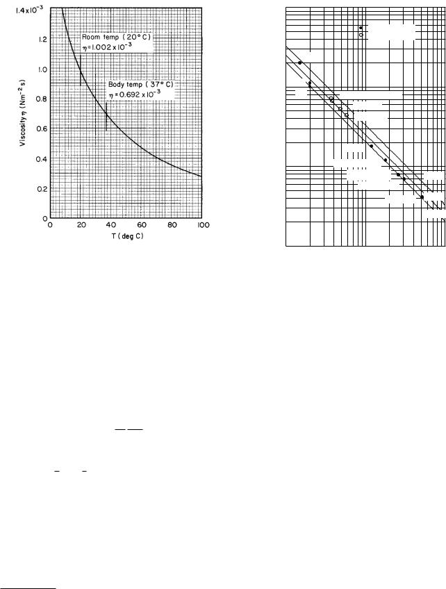
FIGURE 4.10. Viscosity of water at various temperatures. Data are from the Handbook of Chemistry and Physics. (1972), 53rd ed., Cleveland, Chemical Rubber, p. F-36.

It is independent of the nature of the particle or its size. If in addition the di using particles are large enough so that Stokes’ law is valid, then β = 6πηa and9

The di usion constant is inversely proportional to the fluid viscosity and the radius of the particle.

Combining Eqs. 4.18b and 4.22 shows that in terms of the chemical potential,

jsx = −Cβs ∂µ∂xs .

Sometimes minus the gradient of the chemical potential is called the driving force. To see why, note that for solvent drag, js = Csv, so βv = −∂µs/∂x is the driving force.

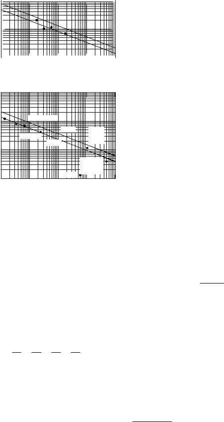
The viscosity of water varies rapidly with temperature, as shown in Fig. 4.10. These values of viscosity and Eq. 4.23 have been used to calculate the solid lines for D vs a shown in Fig. 4.11. Various experimental values are also shown. The di usion constant increases rapidly with temperature, so that care must be taken to specify the temperature at which the data are obtained. Since not all the molecules are spherical, there is some uncertainty in the value of the particle radius a.

9For self-di usion (such as radioactively tagged water in water), a hydrodynamic calculation shows that β = 4πηa [R. B. Bird, W. E. Stewart, and E. N. Lightfoot (1960). Transport Phenomena, New York, Wiley, p. 514 ].

a (nm)

FIGURE 4.11. Di usion constant versus sphere radius a for di usion in water at three di erent temperatures. Experimental data at 20 ◦C (293 K) are from Benedek and Villars (2000), Vol. 2, p. 122. Data at 25 ◦C (298 K) are from Handbook of Chemistry and Physics, (1972), 53rd ed., Cleveland, Chemical Rubber, p. F-47.

Figure 4.12 is a plot of D for particles di using in water at 20 ◦C (293 K) vs. molecular weight M . Although the solid line provides a rough estimate of D if M is known, scatter is considerable because of varying particle shape. DNA lies a factor of 10 below the curve, presumably because it is partially uncoiled and presents a larger size than other molecules of comparable molecular weight.

It is possible to measure the self-di usion of water in water by using a few water molecules in which one hydrogen atom is radioactive and measuring how they di use. Water has an unusually large self-di usion constant.

If all of the molecules shown had the same density, then their radius would depend on M 1/3 and the line would have a slope of −13 . The slope is steeper than this, suggesting that the molecules are larger for large M than constant density would predict. This increase in size may be partially attributable to water of hydration. The precise values of di usion constants depend on many details of the particle structure; however, the lines in Fig. 4.12 provide an order-of-magnitude estimate.

The assumption that the flux depends linearly on the concentration gradient was an approximation. The di u- sion constant is found, as a result, to be somewhat concentration dependent.

Molecular weight M (Dalton)

Molecular weight M (Dalton)

FIGURE 4.12. Di usion constant versus molecular weight in daltons. (One dalton is the mass of one hydrogen atom.) Data at 293 K are from Benedek and Villars (2000), Vol. 2, p. 122. The 293-K solid line was drawn by eye through the data; the line at 310 K was drawn parallel to it using the temperature change in Eq. 4.23. Data scatter around the line by about 30%, with occasional larger departures.

right-hand side of Eq. 4.24,

is called the Laplacian of C. It is often abbreviated as2C (read “del squared C”) in American textbooks or ∆C in European books. It is given in other coordinate systems in Appendix L.

In principle, if C(x, y, z) is known at t = 0, Eq. 4.24 can be solved for C(x, y, z, t) at all later times. (We develop a general, and sometimes useful, equation for doing this below.) We may also look at this equation as a local equation, telling how C changes with time at some point if we know how the concentration changes with position in the neighborhood of that point. The change of concentration with position determines the flux j. The changes in flux with position determine how the concentration changes with time.

There is extensive literature on how to solve the diffusion equation (or the heat-flow equation, which is the same thing).10 Instead of discussing a large number of techniques, we show by substitution that a Gaussian or normal distribution function, spreading in a certain way with time, is one solution to Eq. 4.24. In Sec. 4.14 we independently derive the same solution from a random-walk model of di usion. An important feature of the Gaussian solution is that the center of the distribution of concentration does not move.

For simplicity, consider the one-dimensional case. Take the distribution to be centered at the origin and find those conditions under which11

4.8 Fick’s Second Law of Di usion

Fick’s first law of di usion, Eq. 4.18a, is the observation that for small concentration gradients, the di usive flux density is proportional to the concentration gradient: jx = −D ∂C/∂x. If this is di erentiated, one obtains ∂jx/∂x = −D ∂2C/∂x2. Similar equations hold for the y and z directions. The equation of continuity, Eq. 4.2, is

−∂C∂t = ∂j∂xx + ∂j∂yy + ∂j∂zz .

If we combine these two equations, we get Fick’s second law of di usion, also known as the di usion equation:

The first law relates the flux of particles to the concentration gradient. The second law tells how the concentration at a point changes with time. It combines the first law and the equation of continuity. The function on the

2πσ(t)

We can view the one-dimensional case in either of two ways. If it represents di usion along a pipe, then C(x, t) is the number of particles per unit length in a slice between x and x+dx, and N is the total number of particles. If it represents a three-dimensional problem with concentration changing only in the x direction, then C(x, t) is the number of particles per unit volume and N is the number of particles per unit area.

Equation 4.25 is a solution to the one-dimensional version of Eq. 4.24:

10See, for example, Crank (1975) or Carslaw and Jaeger (1959).

11The properties of the Gaussian function, Eq. 4.25, are discussed in Appendix I.

92 4. Transport in an Infinite Medium

To do this, we will need various derivatives of Eq. 4.25. They can be evaluated using the chain rule:

When these are substituted in Eq. 4.26, the result is

We can divide both sides of this equation by

because this factor is never zero. The result is

We can divide by x2/σ2 − 1 for all values of x except x = ±σ. These values of x are where the second derivative of C vanishes; at these points, ∂C/∂t = 0 for any value of σ. At all other points, the solution will satisfy the equation only if

σ dσdt = D.

This can be integrated to give

σ dσ = D dt

or

12 σ2(t) = Dt + const.

Multiply through by 2 and observe that σ2(0) = 2 const, so that

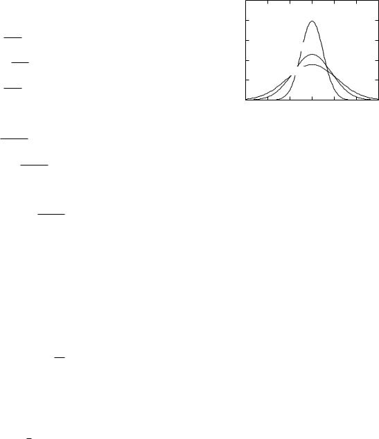
If the concentration is initially Gaussian with variance σ2(0), after time t it will still be Gaussian, centered on the same point, with a larger variance given by Eq. 4.27. Figure 4.13 shows this spreading in a typical case. At still earlier times the concentration would have been even more narrowly peaked. In the limit when σ(t) is zero, all the particles are at the origin, giving an infinite concentration. This is, of course, impossible. However, all the particles could be very close to the origin, giving a very tall, narrow curve for C(x).

The width of the curve, determined by σ, increases as the square root of the time. A square root increase is

FIGURE 4.13. Spreading of particles by di usion assuming D = 1.

less rapid than a linear increase, reflecting the fact that as the particles spread out the concentration does not change as rapidly with distance, so that the flux and the rate of spread decrease.

Note that the rate of change of concentration with time depends on the second derivative of the concentration with distance. This is because the rate of buildup is the flux into a region at some surface minus the flux out through a nearby surface; each flux is proportional to the gradient of the concentration, so the buildup is proportional to the di erence in gradients or the second derivative.

In the Problems at the end of this chapter you will discover that di usion of small particles through water for a distance of 1 µm takes about 1 ms, and di usion through 100 µm takes 1002 times as long, or 10 s. The times are even longer for larger particles. Thus, di usion is an effective mode of transport for distances comparable to the size of a cell, but it is too slow for larger distances. This is why multicelled organisms evolve circulatory systems.

4.9 Time-Independent Solutions

In this section we develop general solutions for di u- sion and solvent drag when particles are conserved and the concentration and fluence rate are not changing with time. The system is in the steady state. The continuity equation, Eq. 4.8, then becomes div j = 0. We consider the solutions for C and j in one, two, and three dimensions when the symmetry is such that j depends on only one position coordinate, x or r. These solutions are sometimes appropriate models for limited regions of space. There is always some other region of space, serving as a source or sink for the particles that are di using, where the model does not apply.

The behavior of j can be deduced from the continuity equation. In one dimension, such as flow in a pipe or between two infinite planes, the continuity equation is

which has a solution jx = b1 where b1 is a constant. (The subscript denotes the constant for the one-dimensional case.) The total flux or current i is constant, so

where S is the area perpendicular to the flow.

In two dimensions, we consider a problem with cylindrical symmetry and consider only flow radially away from or towards the z axis. In that case, the equation in Table

This is valid everywhere except along the z axis, where there is a source of particles and the divergence is not zero. The total current i leaving a region of length L parallel to the z axis is also constant,

In three dimensions with spherical symmetry, the ra-

This is valid everywhere except at the origin, where there is a source of particles.

These results depend only on continuity, time independence, and the assumed symmetry. They are true for diffusion, solvent drag, or any other process. Note the progression in going to higher dimensions: in n dimensions rn−1jr is constant.

Now consider how the concentration varies in the two limiting cases of pure solvent drag and pure di usion. (Section 4.12 discusses what happens when both transport modes are important.)

For solvent drag, the velocity of the solvent is the volume flux density jv which also satisfies the continuity equation. In one dimension jv = iv /S. In two dimensions

jv = iv /2πLr, and in three dimensions jv = iv /4πr2. In each case

Since Cs is constant, there is no di usion.

For the case of di usion, j = −D C. In one dimension

this becomes

dCdx = −SDi , which is integrated to give

i

C = −SD x + b1,

where b1 is the constant of integration. The concentration varies linearly in the one-dimensional case. If i is positive (flow in the +x direction), C decreases as x increases. Often the concentration is known at x1 and x2, and one

We can again solve for the current when the concentrations are known at two di erent radii:

Di usion in two dimensions with cylindrical symmetry has been used to model the concentration of substances in the region between two capillaries.

The three-dimensional case is worth further discussion, because it can help us to understand the di usion of nutrients to a single spherical cell or the di usion of metabolic

i = 4πD C0R,

C(r) = C0R , r

C0DR jr = r2 .

(4.39a)

(4.39b)

(4.39c)

The particle current depends on the radius of the cell, R, not on R2. This very important result is not what we might naively expect. Di usion-limited flow of solute in or out of the cell is proportional not to the cell surface area, but to the cell radius. The reason is that the particle movement is limited by di usion in the region around the cell, and as the cell radius increases, the concentration gradient decreases. (It is possible for the rate of particle migration into the cell to be proportional to the surface area of the cell if some other process, such as transport through the cell membrane, is the rate-limiting step.)

If di usion is toward the cell, the concentration is C0 infinitely far away. At the cell surface, every di using molecule that arrives is assumed to be captured, and the concentration is zero. The solutions are then

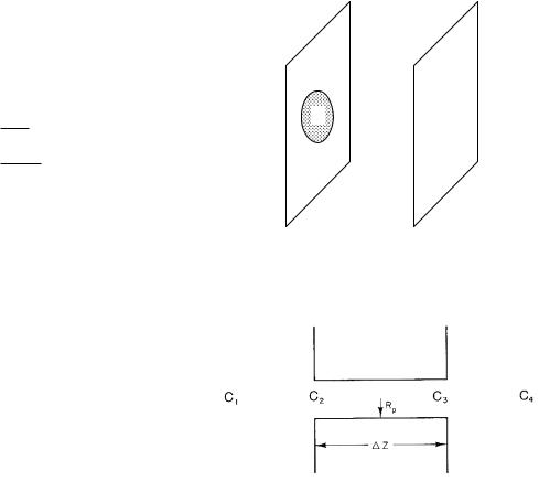
FIGURE 4.14. The di usion flux from the disk of radius a and concentration C1 to the infinite sheet where the concentration is C2 is given by i = 4Da(C1 − C2).

4.10Example: Steady-State Di usion to a Spherical Cell and End E ects

In the preceding section we considered di usion from infinitely far away to the surface of a spherical cell where the concentration was zero. We now add the e ect of steadystate di usion through a series of pores or channels in the cell membrane. This will lead to a very important result: it does not require very many pores per unit area in the cell membrane to “keep up with” the rate of di usion of chemicals toward or away from the cell. The result is important for understanding how cells acquire nutrients, how bacteria move in response to chemical stimulation (chemotaxis), and how the leaves of plants function.

To develop the model we need one more result: the current due to di usion from a disk of radius a where the concentration is C1 to a plane far away where the concentration is C2. The disk is embedded in the surface of an impervious plane as shown in Fig 4.14, so particles cannot cross to the region behind the disk. The current is (Eq. 6.98)

FIGURE 4.15. End e ects in di usion through a pore.

It is proportional to the radius of the disk, not its surface area. [Obtaining this result requires solving the di usion equation in three dimensions. See Carslaw and Jaeger (1959), p. 215.]

Consider di usion through a pore of radius Rp which pierces a membrane of thickness ∆Z, including di usion in the medium on either side of the membrane (Fig. 4.15). If the material on either side were well stirred, there would be a uniform concentration C1 on the left and C4 on the right. Because it is not stirred, there is di usion in the exterior fluid. Let C1 and C4 be measured far away, and call the concentrations at the ends of the pore C2 on the left and C3 on the right.

Equation 4.38a gives the di usion flux within the pore

In the steady state, there is no buildup of particles and i is the same in each region. We can solve Eqs. 4.42–4.44