

Intermediate Physics for Medicine and Biology - Russell K. Hobbie & Bradley J. Roth
.pdf7.7 The Electrocardiographic Leads |
187 |
FIGURE 7.17. The three components of the total current-di- pole vector p as a function of time.
FIGURE 7.18. Geometry for calculating the potential di erence due to p between points A and B.
The potential di erence between two electrodes separated by a displacement R and equidistant from the currentdipole vector p measures the instantaneous projection of vector p on R.
If the depolarization can be described by a single current-dipole vector, only three measurements are needed in principle, corresponding to the projections on three perpendicular axes. The standard electrocardiogram (ECG) records 12 potential di erences using nine electrodes. There are many reasons for this. The body is not an infinite, homogeneous conductor, and the relationship between cellular dipole moments and the potential is more complicated than our model; to convert the three perpendicular components to the instantaneous values of p would require a mathematical reconstruction; and the
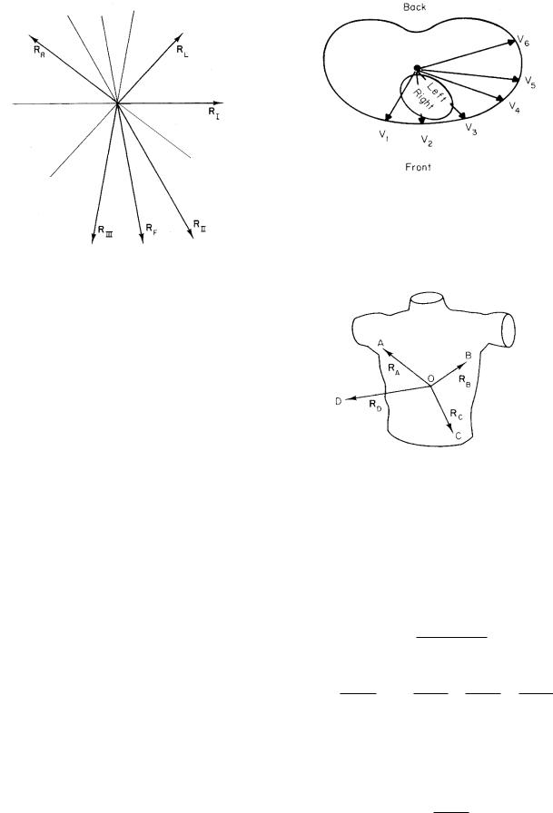
FIGURE 7.19. Vectors connecting the three electrodes for a typical patient. The limbs are extensions of the leads of the electrocardiograph machine.
electrodes are not far away compared to the size of the heart. With 12 recorded potential di erences, it is fairly easy to interpret the electrocardiogram by inspection.
The first three electrodes are placed on each wrist and the left leg. The limbs serve as extensions of the wires, so that the potential is measured where the limbs join the body. This is a major correction to our crude model that the heart is in an infinite conducting medium. If the subject were immersed in a conducting medium such as sea water, movement of the arms would change the size of the ECG signal because it would change R. In air, however, movement of the arms does not change the size of the signal. The simplest correction to explain this is to say that R for the two arm electrodes goes from shoulder to shoulder. These three electrodes measure potential di erences between three points located approximately as shown in Fig. 7.19. The dimensions are for a typical adult. The three potential di erences are called limb leads I, II, and III:
I = vB − vA,
II = vC − vA, |
(7.31) |
III = vC − vB .
In the approximation used here, the voltage di erence I is proportional to the projection of p on RI, and so forth. These leads measure the projections of p on the three vectors RI, RII, and RIII of Fig. 7.19.
It is customary also to combine these three potentials in a slightly di erent way to obtain projections of p on three other directions. These combinations are called the augmented limb leads. They contain no information that was not already present in the limb leads, but the six
188 7. The Exterior Potential and the Electrocardiogram
FIGURE 7.20. The six directions in the frontal plane defined by the limb leads and the augmented limb leads. The angles are for the same subject as in Fig. 7.19.
signals are easier to interpret by inspection. The combinations are
|
|
|
1 |
|
|
|
|
1 |
|
|
|||
aV R = vA − |
|
|
(vB + vC ) = − |
|
(I + II), |
|
|||||||
2 |
2 |
|
|||||||||||
1 |
|
|
|
|
1 |
|
|
|
|
|
|
||
aV L = vB − |
|
(vA + vC ) = |
|
|
(I − III), |
(7.32) |
|||||||
2 |
2 |
||||||||||||
aV F = vC − |
1 |
(vA + vB ) = |
1 |
(II + III). |
|
||||||||
|
|
|
|
||||||||||
2 |
2 |
|
|||||||||||
These are proportional to the projections of p on vectors RL, RR, and RF of Fig. 7.20. The subscripts refer to the fact that the vectors point toward the left shoulder, right shoulder, and foot, respectively.
The six lines in Fig. 7.20 are spaced approximately every 30 ◦ in the frontal plane. Many texts argue that the leads are spaced exactly every 30 ◦ and that the triangle of Fig. 7.19 is an equilateral triangle (Einthoven’s triangle). While the directions are not far from 30 ◦, this assumption is not really necessary. Physicians often want to know the direction of p at some point during the cardiac cycle, or the average direction of p during the QRS wave (ventricular depolarization). With six directions measured, this can be determined by inspection.
These six leads measure projections in the frontal plane. It is also necessary to have at least one projection in a plane perpendicular to the frontal plane. It is customary to place six leads across the chest wall in front of the heart; they are called the precordial leads. Their locations are shown in Fig. 7.21. The potential di erence is measured between each precordial electrode and the average of vA, vB , and vC . A lead therefore measures the projection of p on a vector from the center of triangle ABC to the electrode for that lead. This fact is not obvious, and in fact is true only if di erences in 1/r2 are neglected. To
FIGURE 7.21. The location of the precordial leads and the directions of the components of p which they measure. Reprinted with permission from R. K. Hobbie. The electrocardiogram as an example of electrostatics. Am. J. Phys. 41: 824–831. Copyright 1973, American Association of Physics Teachers.
FIGURE 7.22. A perspective drawing of the vectors used to calculate the potential in a precordial lead. Reprinted with permission from R. K. Hobbie. The electrocardiogram as an example of electrostatics. Am. J. Phys. 41: 824–831. Copyright 1973, American Association of Physics Teachers.
see that it is true with the appropriate approximation, pick an arbitrary point O and from it construct vectors RA, RB , RC , and RD to the points A, B, and C of Fig. 7.22 and to the precordial electrode at D. The desired potential is
v = vD − vA + vB + vC .
3
It can be calculated using Eq. 7.30 for each term:
v = |
1 |
p · RD |
− |
1 |
|
p · RA |
+ |
p · RB |
+ |
p · RC |
. |
4πσo RD3 |
|
|
RB3 |
|
|||||||
|
3 RA3 |
|
|
RC3 |
|||||||
So far, the location of O is arbitrary. If it is picked to be at the center of the triangle, then RA + RB + RC = 0. (This is the definition of center.) Since RA ≈ RB ≈ RC , the term in large parentheses vanishes. The desired potential di erence is then
v = |
1 |
|
p · RD |
. |
4πσo |
|
|||
|
|
RD3 |
||
7.8 Some Electrocardiograms |
189 |
In this approximation, each precordial lead measures the projection of p on a vector from the center of the triangle ABC to the electrode. The amplitude of the signal will be larger than for the limb leads, because RD < RA. Some of the precordial leads are quite close to the heart. The assumption that r is the same for all parts of the myocardium is not valid. Because of the factor 1/r2, the greatest contribution to the potential comes from the closest regions of myocardium. A lead is said to “look at” the myocardium closest to it.
7.8 Some Electrocardiograms
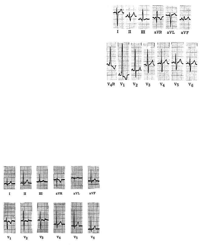
A normal electrocardiogram is shown in Fig. 7.23. When p has its greatest magnitude during the QRS wave, it is nearly parallel to RII. There is almost no signal in aV L, which is perpendicular to RII.
Compare this to Fig. 7.24, which shows the electrocardiogram for a patient with right ventricular hypertrophy, an enlargement and thickening of the right ventricle. Because of the greater right ventricular muscle volume, p points to the right during the QRS wave, so that the QRS signal is negative in lead I. Lead aV F shows that there is very little vertical component of p during the QRS wave. The precordial leads V1 and V2 show the strongest signals, because the right ventricle faces the front of the body. In this case an extra lead V4R has been used, which is symmetrical with V4 but on the right side of the body.
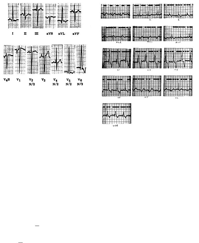
The electrocardiogram in Fig. 7.25 is from a patient with left ventricular hypertrophy. The thicker left ven-
FIGURE 7.24. The electrocardiogram of a patient with right ventricular hypertrophy. Reprinted with permission from R. K. Hobbie. The electrocardiogram as an example of electrostatics. Am. J. Phys. 41: 824–831. Copyright 1973, American Association of Physics Teachers. The electrocardiogram was supplied by Prof. James H. Moller, M.D.
tricular wall causes the QRS dipole to point to the left. As a result, lead I has an abnormally high peak, aV L is large and positive, V2 is negative, and V4, V5, and V6 have very large positive peaks. These last four leads are shown at half scale.
A fault in the conduction system known as a bundle branch block causes the depolarization wave to travel through the myocardium rather than over the conduction system. Since the speed of propagation in myocardium is slower than that in the conduction system, the depolarization takes longer than usual. An electrocardiogram for a patient with right bundle branch block (a block in the bundle for the right ventricle) is shown in Fig. 7.26. The e ect is most striking in leads that are most sensitive to the right ventricle: precordial leads 1 and 2. In V1 the early part of the QRS wave has the usual biphasic, up–down pattern as the left ventricle depolarizes. This is followed by a large and prolonged vector pointing to the right, as the right ventricle slowly depolarizes. Lead V2 shows a strong and prolonged bipolar signal as the right ventricle depolarizes.
FIGURE 7.23. A normal electrocardiogram. The large divisions are 0.5 mV vertically and 0.2 s horizontally. Reprinted with permission from R. K. Hobbie. The electrocardiogram as an example of electrostatics. Am. J. Phys. 41: 824–831. Copyright 1973, American Association of Physics Teachers. The electrocardiogram was supplied by Prof. James H. Moller, M.D.
7.9 Refinements to the Model
Our model for the potential outside a nerve or muscle cell has been a long single conducting fiber in an infinite, homogeneous medium. We will consider four ways to extend and improve the model. The first is to recognize that current must also flow radially inside the cell. If it did not, it
190 7. The Exterior Potential and the Electrocardiogram
FIGURE 7.25. The electrocardiogram for a patient with left ventricular hypertrophy. Reprinted with permission from R. K. Hobbie. The electrocardiogram as an example of electrostatics. Am. J. Phys. 41: 824–831. Copyright 1973, American Association of Physics Teachers. The electrocardiogram was supplied by Prof. James H. Moller, M.D.
could never leave the cell. At the same time we will abandon the assumption that the presence of the cell along the x axis does not perturb the current outside the cell. The third improvement is to recognize that the conductivity may depend on position. This is particularly important outside the cell, where there are muscle, fat, lungs, etc. Finally, the conductivity at a given point may depend on which direction the current flows—for example, parallel or perpendicular to the cells.
In order to make these refinements to the model, we must develop a di erent formulation of the problem. Consider some region of space containing a conducting material described by Ohm’s law. The electric field is related to the potential by Eq. 6.16b: E = −grad v = −v. If the material is isotropic and obeys Ohm’s law, then from Eq. 6.26
j = σE = −σ v. |
(7.33) |
We now apply the equation of continuity or conservation of charge, casting Eq. 4.8 in terms of the electric current density j and the electric charge per unit volume, ρ:
∂ρ |
= − · j. |
(7.34) |
∂t |
Combining these two equations gives
∂ρ |
= div(σ grad v) = · (σ v). |
(7.35) |
∂t |
Leaving the conductivity inside the divergence term allows the conductivity to depend on position. If the conductivity is the same everywhere it can be taken outside
FIGURE 7.26. The electrocardiogram for a patient with right bundle branch block. The electrocardiogram was supplied by Prof. James H. Moller, M.D.
the divergence operator to give |
|
|
|
|
|||||||
|
∂ρ |
2 |
|
∂2v |
∂2v |
|
∂2v |
|
|
||
|
|
= σ |
v = σ |
|
|
+ |
|
+ |
|
. |
(7.36a) |
|
∂t |
∂x2 |
∂y2 |
∂z2 |
|||||||
We can write this in cylindrical coordinates which are more useful for modeling a cylindrical cell stretched along the z axis. From Appendix L, assuming that the potential does not depend on the polar angle φ, we have
∂ρ |
2 |
|
1 ∂ |
|
∂v |
|
∂2v |
|
||||
|
= σ |
v = σ |
|
|
|
r |
|
|
+ |
|
|
. (7.36b) |
∂t |
r ∂r |
∂r |
|
∂z2 |
||||||||
These are very general equations, applicable to any volume of space where the material is homogeneous and isotropic and obeys Ohm’s law. They were derived using Ohm’s law and the conservation of charge. Equation 7.36a is actually the same result we had in Eq. 6.51. This is demonstrated in Problem 29.
7.9.1 The Axon Has a Finite Radius
Now we can make the first two improvements: we relax the assumption that the axon radius is very small. Except
at the cell membrane, where charge on the membrane capacitance is changing as the membrane potential changes, ∂ρ/∂t = 0. If we assume that the transmembrane potential vm is known, then Eq. 7.36b can be applied separately to the extracellular and the intracellular fluid for a long straight axon to determine the potential everywhere outside (or inside). This was first done by Clark and Plonsey (1968). In the extracellular and intracellular fluids, Eq. 7.36b becomes
1 ∂ |
r |
∂vo(r, z) |
|
+ |
∂2vo(r, z) |
= 0, |
r > a |
|
||||||
|
|
|
|
|
|
|
|
|
|
|||||
r ∂r |
|
∂r |
∂z2 |
|
||||||||||
|
|
|
|
|
|
|||||||||
|
1 ∂ |
r |
|
∂vi(r, z) |
|
+ |
∂2vi(r, z) |
= 0, |
r < a |
(7.37) |
||||
|
|
|
|
|
|
|
|
|
||||||
|
r ∂r |
|
∂r |
∂z2 |
|
|||||||||
|
|
|
|
|
|
|
||||||||
vm(z) = vi(a, z) − vo(a, z).
With vm known, these equations were solved for the potential distribution inside and outside the cell. This is the calculation that was done to obtain Fig. 7.13. The result of this type of calculation has been compared to the line-source model by Trayanova et al. (1990).
7.9.2 Nonuniform Exterior Conductivity
To make the next improvement, consider an extracellular region in which the conductivity is not uniform. In a region without sources, the potential obeys
· (σo vo) = 0. |
(7.38) |
Often, the conductivity is assumed to be “piecewise” homogenous, with a di erent value assigned to each kind of tissue. Within each tissue the potential then obeys Laplace’s equation, 2vo = 0. At the boundary between tissues, the potential and the normal component of the current are continuous.
When the di erent tissues have realistic and irregular boundaries, special techniques are needed to solve Laplace’s equation. One important technique is the “finite-element method” [Miller and Henriquez (1990)], and another is the “boundary-element method” [Gulrajani (1998)].
A typical application, which serves as the basis for “noninvasive electrocardiographic imaging,” is to measure the potential at the body surface and then calculate the potential on the epicardium (the outer surface of the heart)[Rudy and Burnes (1999); Stanley et al. (1986)]. One cannot calculate the potential inside the heart unless the sources are known, but finding the potential on the epicardial surface is possible.
7.9.3Anisotropic Conductivity: The Bidomain Model
The final improvement recognizes that the cardiac tissue is generally not isotropic. If it is still described by Ohm’s
7.9 Refinements to the Model |
191 |
law, then we can write j = σ. · E where σ. is a matrix or tensor. In Cartesian coordinates
jx |
σxx |
σxy |
σxz |
Ex |
|
jy |
= σyx |
σyy |
σyz |
Ey |
. (7.39) |
jz |
σzx |
σzy |
σzz |
Ez |
|
This is a compact notation for
jx = σxxEx + σxy Ey + σxz Ez ,
with similar equations for jy and jz . It can be shown that the conductivity matrix must be symmetric, so there are actually six conductivity coe cients, not nine. It is often possible to make some of the matrix elements zero by suitable choice of a coordinate system and suitable orientation of the axes.
Problem 29 shows that for a small cylindrical region of isotropic axoplasm of length h and radius a, the cylindrical surface of which is surrounded by cell membrane, the total charge Q within the axoplasm changes according to
|
∂Q |
= πa2h |
∂ρi |
= C |
|
∂vm |
+ im = 2πah cm |
∂vm |
|
+ jm |
, |
||||||||||||||
|
∂t |
∂t |
|
|
|
∂t |
|||||||||||||||||||
|
|
|
|
|
∂t |
|
|
|
|
|
|
|
|
|
|
|
|||||||||
or |
|
∂vm |
|
|
|
|
πa2h |
|
|
∂2vi |
|
|
σia |
|
∂2vi |
|
|
|
|
||||||
|
|
cm |
+ jm = |
σi |
= |
|
. |
|
|
||||||||||||||||
|
|
|
∂t |
|
|
∂x2 |
|
|
|
|
|
||||||||||||||
|
|
|
|
|
|
2πah |
|
|
2 |
|
|
∂x2 |
|
|
|||||||||||
This can also be written as |
|
|
|
|
|
|
|
|
|
|
|
|
|
|
|||||||||||
|
|
|
|
|
|
|
∂vm |
|
|
∂2vi |
|
|
|
|
|
||||||||||
|
|
|
|
β cm |
|
+ jm |
|
= σi |
|
, |
|
|
|
|
|
||||||||||
|
|
|
|
∂t |
|
∂x2 |
|
|
|
|
|
||||||||||||||
where β = 2πah/πa2h = 2/a is the ratio of surface area to volume of the cell. Our cell was cylindrical. With other geometrical configurations, such as a cubic or a spherical cell, β would have a di erent value, but it always has the dimensions of (length)−1. In the general threedimensional anisotropic case, the equivalent equation is
β |
cm |
∂vm |
+ jm |
(7.40) |
|
∂t |
|||||
|
|
|
|
zero, except at the cell membrane
= div(σ.i grad vi) = · (σ.i vi)
Both σi and vi are functions of position. The left-hand side is zero except at the cell membrane. The main theme of this chapter has been that current that stops flowing inside the cell must flow outside the cell. We can write an analogous equation for the region outside the cell:
|
|
∂vm |
+ jm |
|
−β |
cm |
|
= div(σ.o grad vo) (7.41) |
|
∂t |
zero, except at the cell membrane
= · (σ.o vo)
Myocardial cells are typically about 10 µm in diameter and 100 µm long. They have the added complication that they are connected to one another by gap junctions, as shown schematically in Fig. 7.27. This allows currents to

192 7. The Exterior Potential and the Electrocardiogram
v i (r,t )
vo (r,t )
FIGURE 7.27. The interior of myocardial cells (shaded) is connected to adjoining cells by gap junctions. The bidomain model assumes that in a small region of space (large compared to a cell) there are two potentials: the interior potential and outside potential that are functions of position and time.
The membrane current jm can be modeled by either a passive membrane (Ohm’s law—electrotonus) or with one of the models for an active membrane.
Anisotropy plays an important role in the bidomain model. To see why, consider a solution to Laplace’s equation in a monodomain—a two-dimensional sheet of homogeneous, anisotropic tissue with straight fibers. If the x direction is chosen to be along the fiber direction (the direction of greatest conductivity), then Laplace’s equation becomes
σox |
∂2vo |
+ σoy |
∂2vo |
= 0. |
2 |
2 |
|||
|
∂x |
|
∂y |
|
Now define a new set of coordinates x = x and y =
#
σox/σoy y. You can show that in these new coordinates Laplace’s equation becomes
∂2vo + ∂2vo = 0. ∂x 2 ∂y 2
flow directly from one cell to another without flowing in |
We have removed the e ect of anisotropy by rescaling |
||||||||||||||||
the extracellular medium. The bidomain (two-domain) |
distance in the direction perpendicular to the fibers. If |
||||||||||||||||
model is often used to model this situation [Henriquez |
you try a similar trick with the bidomain model |
||||||||||||||||
(1993)]. It considers a region, small compared to the size |
|
∂2vi |
|
∂2vi |
|
|
∂vm |
|
|
||||||||
of the heart, that contains many cells and their surround- |
|
|
|
|
|
|
|
|
|
|
|
|
|
|
|
|
|
σix ∂x2 |
+ σiy ∂y2 |
= β |
cm ∂t + jm |
(7.44a) |
|||||||||||||
ing extracellular fluid. It simplifies the problem by assum- |
|||||||||||||||||
ing that each small volume element contains two domains, |
∂2vo |
∂2vo |
|
|
|
∂vm |
|
|
|||||||||
intracellular and extracellular. |
σox |
|
|
+ σoy |
|
|
= −β |
|
cm |
|
+ jm , |
(7.44b) |
|||||
∂x2 |
|
∂y2 |
|
|
∂t |
||||||||||||
Think of the volume element as the entire region shown |
you can find a new coordinate system that removes the |
||||||||||||||||
in Fig. 7.27. There are two potentials in each small vol- |
|||||||||||||||||
e ect of anisotropy in either the intracellular |
space or |
||||||||||||||||
ume element: vi(r, t) and vo(r, t). These potentials are |
|||||||||||||||||
the extracellular space, but in general you cannot find a |
|||||||||||||||||
averages over the intracellular and extracellular domains |
|||||||||||||||||
coordinate system that removes the anisotropy in both |
|||||||||||||||||
contained in the volume element. The transmembrane |
|||||||||||||||||
spaces simultaneously [Roth (1992)]. Only in the special |
|||||||||||||||||
potential is the di erence between these two potentials: |
|||||||||||||||||
case of equal anisotropy ratios (σix/σiy = σox/σoy ) will |
|||||||||||||||||
vm(r, t) = vi(r, t) − vo(r, t). Charge can pass freely be- |
|||||||||||||||||
the equations simplify dramatically. But the anisotropy |
|||||||||||||||||
tween the two domains, but the total charge within a |
ratios in the heart are not equal. In the intracellular space |
||||||||||||||||
volume element is conserved. If the current densities in |
|||||||||||||||||
the ratio of conductivities parallel and perpendicular to |
|||||||||||||||||
each domain are ji and jo, then the divergence of the sum |
|||||||||||||||||
the fibers is about 10:1, while in the extracellular space |
|||||||||||||||||
is zero: · (ji + jo) = 0. The divergence of each current |
|||||||||||||||||
this ratio is about 4:1 [Roth (1997)]. Anisotropy plays |
|||||||||||||||||
individually passes through the membrane or charges the |
|
|
|
|
|
|
|
|
|
|
|
|
|
|
|
|
|
membrane capacitance. The anisotropic analogs of Eqs. |
an essential role in the electrical behavior of the heart, |
|
especially during electrical stimulation. |
||
7.40 and 7.41 are now |
||
|
|
∂vm |
|
|
|
|
|
||
β |
cm |
|
+ jm |
= div(σ.i · grad vi) = · (σ.i · vi), |
||||
∂t |
||||||||
|
|
|
|
∂vm |
+ jm |
|
||
|
|
−β |
|
cm |
|
|
= div(σ.o · grad vo) |
|
|
|
|
∂t |
|
||||
= · (σ.o · vo).
(7.42) The quantity β is the membrane surface area per unit volume of the entire bidomain—both intracellular and extracellular volumes. For example, if we consider that the cells are all cylindrical of length h and radius a, then the surface area of a cell is 2πah. If the fraction of the total volume occupied by cells is f , then the total volume associated with this cell is πa2h/f , so
β = |
2f |
. |
(7.43) |
|
|||
|
a |
|
|
7.10 Electrical Stimulation
The information that has been developed in this chapter can also be used to understand some of the features of stimulating electrodes. These may be used for electromyographic studies, for stimulating muscles to contract, for a cochlear implant to partially restore hearing, for cardiac pacing, and even for defibrillation. The electrodes may be inserted in cells, placed in or on a muscle, or placed on the skin.
In addition to the material in this section, see Problems 38–41.
A pulse of current is sent to the stimulating electrode. The current required to produce a response depends on

the shape and size of the electrode, its placement, the kind of cell being stimulated, and the duration of the pulse. For a given electrode geometry the shorter the pulse, the larger the current required for a tissue response. For very long pulses there is a minimum current required to stimulate that is called rheobase. The strength-duration curve was first discovered by G. Weiss in 1901. He expressed it in terms of total charge in the stimulating pulse. A description of the strength-duration curve and its history has been given by Geddes and Bourland (1985). They also describe some techniques for making accurate measurements. The strength-duration curve for current was first described by Lapicque (1909) as
i = iR |
1 + |
tC |
, |
(7.45) |
|
t |
|||||
|
|
|
|
where i is the current required for stimulation, iR is the rheobase, t is the duration of the pulse, and tC is chronaxie, the duration of the pulse that requires twice the rheobase current.
Equation 7.45 provides an empirical fit to the experimental data. We can develop a model to explain it using information from Chapter 6. A nerve fires after a certain departure from the resting potential. Subthreshold behavior can be modeled by electrotonus. Suppose that we inject a stimulating current into a cell at the origin. Equation 6.58 gave the voltage along the axon for a current injected in the cell at the origin after an infinitely long time: v − vr = v0e−|x|/λ. The solution to Problem 32 shows that the current injected is
i0 = 2v0/λri. |
(7.46) |
The quantities λ and ri are defined in Chapter 6. The factor of 2 arises because current flows both ways along the cell. The rheobase current is
iR = 2 |
vthreshold |
. |
(7.47) |
|
|||
|
λri |
|
|
If we assume that the threshold voltage is independent of pulse duration, we can use the curve for x = 0 in Fig. 6.31(c) to relate the minimum current to the pulse duration. As long as the pulse is applied, the voltage will rise along this curve. When the current is turned o , the voltage will start to fall. If the voltage had reached threshold, the cell will fire. This curve is the solution of Eq. 6.55. The solution is [Chapter 6, Problem 34; Plonsey (1969, p. 132)]
|
|
|
! |
|
|
" |
|
t |
|
||
v(0, t) − vr = v0 erf |
|
|
|
, |
(7.48) |
τ |
|||||
where τ is the membrane time constant, κ 0ρm. The error function is defined in Eq. 4.74 and is plotted in Fig. 4.21. The current required for stimulation with an intracellular electrode at the origin is therefore
i = |
2vthreshold |
= |
iR |
(7.49) |
|||||
|
|
|
|
|
|
. |
|||
λri erf(# |
|
) |
erf(# |
|
) |
||||
t/τ |
t/τ |
||||||||
7.10 Electrical Stimulation |
193 |
|
4 |
|
|
|
|
|
|
|
|
3 |
|
|
|
|
|
|
|
R |
2 |
|
|
|
|
|
|
|
i/i |
|
|
|
|
|
|
|
|
|
|
|
|
|
i/iR = 1 + 0.228 τ/t |
|
||
|
1 |
|
|
|
i/iR = erf (t/τ)1/2 |
|
||
|
|
|
|
|
|
|||
|
0 |
0.2 |
0.4 |
0.6 |
0.8 |
1.0 |
1.2 |
1.4 |
|
0.0 |
|||||||
|
|
|
|
|
t/τ |
|
|
|
FIGURE 7.28. The stimulus strength-duration curve plotted for the chronaxie–rheobase model, Eq. 7.45 and for electrotonus, Eq. 7.49.
Chronaxie can be related to the time constant τ by setting i = 2iR:
iR
2iR = . (7.50)
#
erf tC /τ
From a table of values of the error function, we find
tC = 0.228τ. |
(7.51) |
Figure 7.28 compares the standard empirical curve, Eq. 7.45, with this model. The curves are experimentally indistinguishable.
Equation 7.45 is also used for surface electrodes. Table 7.1 shows some experimental values for rheobase and chronaxie. The further the electrode from the tissue being stimulated, the greater the rheobase current that is required.
An electrode that is transferring positive charge to the medium is called an anode. One that is collecting positive
TABLE 7.1. Comparison of values for rheobase and chronaxie for di erent stimulations.
Stimulation |
Rheobase |
Chronaxie |
|
|
(mA) |
(ms) |
|
|
|
|
|
Intracellular, from Table 6.1, |
6.7 ×10⁻⁶ |
0.23 |
|
vthreshold = 15 mV |
|
|
|
Myocardium, from good pacing |
0.1 |
|
|
electrodes |
|
|
|
Motor nerves for inspiration, |
49 |
0.17 |
|
from stimulation of chest wall |
|
|
|
[Voorhees et al. (1992)] |
|
|
|
Myocardium, from stimulation |
204 |
1.82 |
|
of chest wall [Voorhees et al. |
|
|
|
(1992)] |
|
|
|
|
|
|
|
194 7. The Exterior Potential and the Electrocardiogram
Anode
+ |
Extracellular |
|
|
|
Intracellular |
Region of hyperpolarization
Region of depolarization
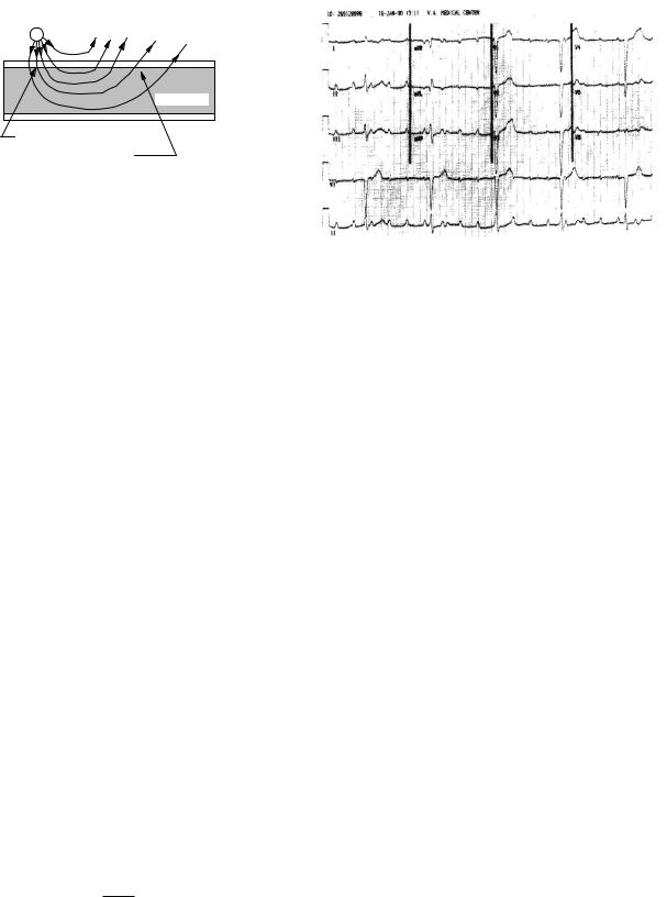
FIGURE 7.29. A schematic drawing showing why there is a region of hyperpolarization near a stimulating anode (positive electrode) with a region of weaker depolarization further away.
charge is called a cathode. If the stimulating electrode is inside the cell, a positive current leaving the electrode will increase the positive charge within the cell and depolarize it. Another way to say it is that current from the electrode flows out through the membrane, so the inside of the membrane will be made more positive than the outside. On the other hand, an anodic electrode just outside the cell will send positive current in through the membrane near the electrode, as shown in Fig. 7.29. This lowers the potential inside and hyperpolarizes the membrane near the electrode. Further away from the stimulation point will be a region where current flows out through the membrane, thus depolarizing the cell. However, the outward current is in general spread out over more membrane, so the current density and hence the depolarization is less than the hyperpolarization near the anode. The situation is, of course, reversed for a cathodic electrode. Figure 7.29 is conceptual; to draw the field lines accurately would require taking into account the conductivities of the extracellular and intracellular fluid as well as the membrane.
The electrotonus model also helps us understand another e ect that is observed: the virtual cathode. The point of origin for a stimulus can be measured by placing sensing electrodes in or on the heart at di erent distances from the stimulating electrode and plotting the time required for the depolarization wave front to reach the electrode vs its position. Extrapolation to the time of stimulus gives the size of the region of initial depolarization. Imagine a stimulating electrode inside a onedimensional cell. When the stimulus current is just above rheobase, the region of depolarization is very small and surrounds the electrode. As the stimulating current is increased, the size of the initial depolarized region grows. From Eqs. 6.58 and 7.50 we obtain
vthreshold = i0λri e−xvc/λ
2
or
|
i0λri |
|
i0 |
|
|
|
xvc = λ ln |
|
|
= λ ln |
|
, |
(7.52) |
2vthreshold |
|
|
||||
|
|
iR |
|
|
||
where xvc is the size of the virtual cathode.
FIGURE 7.30. A patient with third-degree AV heart block. From Rardon, D. P., W. M. Miles, and D. P. Zipes (2000). Atrioventricular block and dissociation. In D. P. Zipes and J. Jalife, eds. Cardiac Electrophysiology: From Cell to Bedside,
3rd ed. Philadelphia, Saunders, pp. 451–459. Used by permission.
Cardiac pacemakers are a useful treatment for certain heart diseases [Je rey (2001), Moses et al. (2000); Barold (1985)]. The most frequent are an abnormally slow pulse rate (bradycardia) associated with symptoms such as dizziness, fainting (syncope), or heart failure. These may arise from a problem with the SA node (sick sinus syndrome) or with the conduction system (heart block ). One of the first uses of pacemakers was to treat complete or “third degree” heart block. The SA node and the atria fire at a normal rate but the wave front cannot pass into the conduction system. The AV node or some other part of the conduction system then begins firing and driving the ventricles at its own, pathologically slower rate. Such behavior is evident in the ECG in Fig. 7.30, in which the timing of the QRS complex from the ventricles is unrelated to the P wave from the atria. A pacemaker stimulating the ventricles can be used to restore a normal ventricular rate.
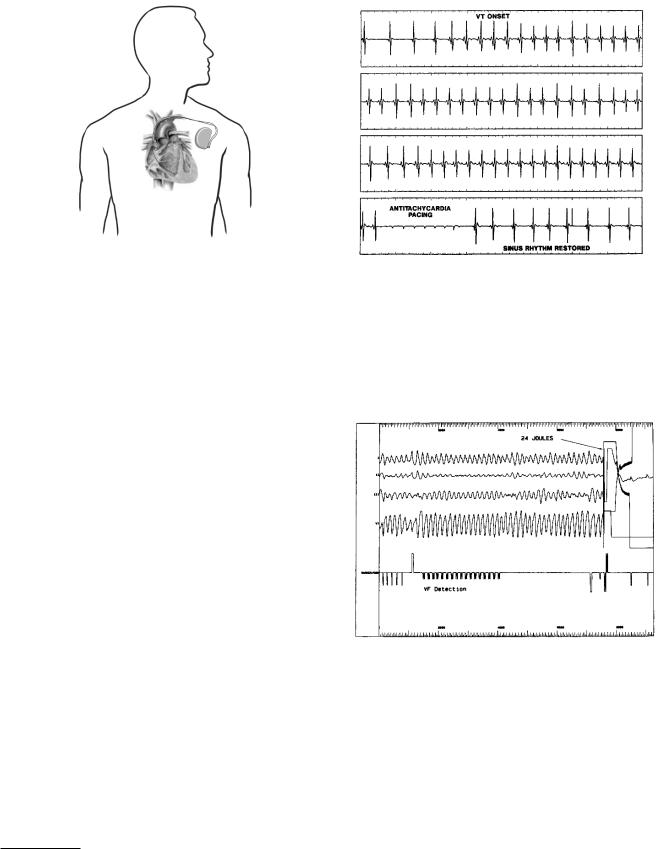
A pacemaker can be used temporarily or permanently. The pacing electrode can be threaded through a vein from the shoulder to the right ventricle (transvenous pacing, Fig. 7.31) or placed directly in the myocardium during heart surgery. Sometimes two pacing electrodes are used, one in the atrium and one in the ventricle. The pacing electrode can be unipolar or bipolar. With a unipolar electrode, the stimulation current flows into the myocardium and returns to the case of the pacemaker, which is often placed in a pocket in the muscle of the chest wall near the shoulder. The return current in a bipolar electrode goes to a ring electrode a few centimeters back along the pacing lead from the electrode at the tip. The surface area of a typical tip is about 10 mm2 (10−5 m2). The current density required to initiate depolarization depends on the spatial distribution of the current and is approximately 100 A m−2. Thus, in this model the current is
7.10 Electrical Stimulation |
195 |
FIGURE 7.31. An implantable pacemaker. The battery and electronics are in a sealed container placed under the skin near the left shoulder. The electrode or “lead” is threaded through the subclavian vein into the right ventricle. Reprinted with permission from Heart and Stroke Facts. p. 29. c 1992–2003 by the American Heart Association.
about8 1 mA. The resistance of the tissue is typically 500 Ω, so the voltage is 0.5 V. After the pacing electrode is implanted, the size of the voltage pulse required to initiate ventricular activity rises because inflammatory tissue grows around the electrode. It is conducting, but the myocardium is further away, and the inflammatory tissue e ectively increases the size of the electrode, thereby reducing the current density. After six months or so, the inflammation has been replaced by a small fibrous capsule, resulting in an e ective electrode size larger than the bare electrode but smaller than the region of inflammation. Recently, electrodes that elute steroids have been used to reduce the inflammation.
Pacemakers can also be designed to detect an abnormal rhythm and apply an electrical stimulus to reverse it. Fig. 7.32 shows a patient with ventricular tachycardia due to a reentrant circuit (p. 186) which has been corrected by pacing very rapidly so that the refractory period prevents the propagation of the reentrant wave.
Ventricular fibrillation occurs when the ventricles contain many interacting reentrant wavefronts that propagate chaotically. Fibrillation is discussed in greater detail in Chapter 10. During fibrillation the ventricles no longer contract properly, blood is no longer pumped through the body, and the patient dies in a few minutes. Implantable defibrillators are similar to pacemakers, but are slightly larger. An implanted defibrillator continually measures the ECG. When a signal indicating fibrillation is sensed, it delivers a much stronger shock that can eliminate the
8Acute implants of smaller electrodes where the electrode resistance is low, as well as computer simulations have shown simulation with currents as small as 18 µA [Lindemans and Denier van der Gon (1978)].
FIGURE 7.32. The top strip shows the onset of ventricular tachycardia, which persists in the next two strips. Very rapid pacing in the fourth strip restores a normal sinus rhythm. Mitrani, R. D., L. S. Klein, D. P. Rardon, D. P. Zipes and W. M. Miles (1995). Current trends in the implantable car- dioverter–defibrillator. In D. P. Zipes and J. Jalife, eds. Cardiac Electrophysiology: From Cell to Bedside, 2nd ed. Philadelphia, Saunders, pp. 1393–1403. Used by permission.
FIGURE 7.33. Ventricular fibrillation has been induced in the electrophysiology laboratory. A pacemaker cardioverter-defib- rillator detects the ventricular fibrillation. A capacitor is then charged and applies a 24-joule defibrillation pulse that restores normal rhythm. Mitrani, R. D., L. S. Klein, D. P. Rardon, D. P. Zipes and W. M. Miles (1995). Current trends in the implantable cardioverter–defibrillator. In D. P. Zipes and J. Jalife, eds. Cardiac Electrophysiology: From Cell to Bedside,
2nd ed. Philadelphia, Saunders, pp. 1393–1403.
reentrant wavefronts and restore normal hearth rhythm (Fig. 7.33).
The bidomain model has been used to understand the response of cardiac tissue to stimulation [Sepulveda et al. (1989); Roth and Wikswo (1994); Roth (1994); Wikswo (1995)]. The former simulation explains a remarkable
196 7. The Exterior Potential and the Electrocardiogram
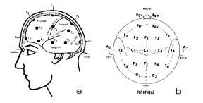
7.34). A typical signal from an electroencephalographic electrode is shown in the top panel of Fig. 11.38. One di culty in interpreting the EEG is the lack of a suitable reference electrode. None of the 21 electrodes in Fig. 7.34 qualifies as a distant ground against which all other potential recordings can be measured. One way around this di culty is to subtract from each measured potential the average of all the measured potentials. In the problems, you are asked to prove that this “average reference
recording” does not depend on the choice of reference
FIGURE 7.34. The standard “10–20” arrangement of elec- electrode; it is a reference independent method. trodes on the scalp for the EEG. Courtesy of Grass, An As-
tro-Med, Inc., Product Group, West Warwick, RI.
experimental observation. Although the speed of the wave front is greater along the fibers than perpendicular to them, if the stimulation is well above threshold, the wavefront originates farther from the cathode in the direction perpendicular to the fibers—the direction in which the speed of propagation is slower. The simulations show that this is due to the anisotropy in conductivity. This is called the “dog-bone” shape of the virtual cathode. It can rotate with depth in the myocardium because the myocardial fibers change orientation. The di erence in anisotropy accentuates the e ect of a region of hyperpolarization surrounding the depolarization region produced by a cathodic electrode. Strong point stimulation can also produce reentry waves that can interfere with the desired pacing e ect.
One of the fundamental problems with research in this area can be seen in equations like 7.42. The variable on the left is the transmembrane potential vm. The variable on the right is the potential inside or outside the cell. Measurement of vm requires measurement or calculation of the di erence vi − vo. Experimental measurements of the transmembrane potential often rely on the use of a voltage-sensitive dye whose fluorescence changes with the transmembrane potential [Knisley et al. (1994); Neunlist and Tung (1995); Rosenbaum and Jalife (2001)].
7.11 The Electroencephalogram
Much can be learned about the brain by measuring the electric potential on the scalp surface. Such data are called the electroencephalogram (EEG). Nunez and Srinivasan (2005) have written an excellent book about the physics of the EEG. We briefly examine the topic here. The EEG is used to diagnose brain disorders, to localize the source of electrical activity in the brain in patients who have epilepsy, and as a research tool to learn more about how the brain responds to stimuli (“evoked responses”) and how it changes with time (“plasticity”). Typically, the EEG is measured from 21 electrodes attached to the scalp according to the “10–20” system (Fig.
Symbols Used in Chapter 7
Symbol |
Use |
Units |
First |
|
|
|
used |
|
|
|
on page |
a |
Axon radius |
m |
179 |
cm |
Membrane |
F m−2 |
191 |
|
capacitance per unit |
|
|
|
area |
|
|
f |
Intracellular volume |
|
192 |
|
fraction |
|
|
h |
Length of segment |
m |
191 |
i |
Current |
A |
178 |
ii, io |
Current inside, |
A |
178 |
|
outside axon |
|
|
iR |
Rheobase current |
A |
193 |
j, j |
Current density |
A m−2 |
178 |
jm |
Current density |
A m−2 |
191 |
|
through membrane |
|
|
p, p |
Activity vector or |
A m |
180 |
|
current dipole |
|
|
|
moment |
|
|
q |
Charge |
C |
178 |
ri |
Resistance per unit |
Ω m−1 |
193 |
|
length inside axon |
|
|
r, r |
Distance |
m |
178 |
t |
Time |
s |
190 |
tC |
Chronaxie |
s |
193 |
v |
Potential |
V |
178 |
vi, vo |
Potential inside, |
V |
191 |
|
outside axon |
|
|
vm |
Potential across |
V |
191 |
|
membrane |
|
|
x, y, z, x0, x1, |
Distance or position |
m |
179 |
x2, y0 |
|
|
|
xvc |
Size of virtual |
m |
194 |
|
cathode |
|
|
C |
Capacitance |
F |
191 |
E, E |
Electric field |
V m−1 |
178 |
Pn |
Legendre polynomial |
|
181 |
Q |
Electric charge |
C |
191 |
R |
Resistance |
Ω |
179 |
R, R |
Distance or position |
m |
182 |
β |
Ratio of surface area |
m−1 |
191 |
|
to volume |
|
|