Intermediate Physics for Medicine and Biology - Russell K. Hobbie & Bradley J. Roth

two or more parameters. If the fitting function is given by y = ax + b, then Q becomes

N

Q = N1 (yj − axj − b)2.

j=1

At the minimum, both ∂Q/∂a = 0 and ∂Q/∂b = 0. The former gives

or

NN

FIGURE 11.2. The best fit to the data of Table 11.1 with the function y = ax + b. Both the slope and the intercept have been chosen to minimize Q.

11.4 become 42a + 10b = 61 and 10a + 3b = 15. These can be easily solved to give a = 1.27 and b = 0.77. The best straight-line fit to the data of Table 11.1 is y = 0.77 + 1.27x. The value of Q, calculated from Eq. 11.2, is 0.013. The best fit is plotted in Fig. 11.2. It is considerably better than the fit with the slope constrained to be one.

A general expression for the solution to Eqs. 11.3 and 11.4 is

!

NN

where x and y are the means. In doing computations where the range of data is small compared to the mean, better numerical accuracy can be obtained from

j=1

11.1.3A Polynomial Fit

The method of least squares can be extended to a polynomial of arbitrary degree. The only requirement is that the number of adjustable parameters (which is one more

288 11. The Method of Least Squares and Signal Analysis

than the degree of the polynomial) be less than the number of data points. If this requirement is not met, the equations cannot be solved uniquely; see Problem 8. If the polynomial is written as

n

y(xj ) = a0 + a1xj + a2x2j + · · ·+ anxnj = akxkj , (11.6)

Index j ranges over the data points; index k ranges over the terms in the polynomial. This expression for Q can be di erentiated with respect to one of the n+1 parameters, say, am:

Setting this derivative equal to zero gives

11.1.4Variable Weighting

The least-squares technique described here gives each data point the same weight. If some points are measured more accurately than others, they should be given more weight. This can be done in the following way. If there is an associated error δyj for each data point, then one can weight each data point inversely as the square of the error and minimize

It is easy to show that the e ect is to add a factor of (1/δyj )2 to each term in the sums in Eqs. 11.8 [Gatland (1993)]. This assumes that errors exist only in the y values. If there are errors in the x values as well, it is possible to make an approximate correction based on an e ective error in the y values [Orear (1982)] or to use an iterative but exact least-squares method [Lybanon (1984)]. The treatment of unequal errors has been discussed by Gatland (1993) and by Gatland and Thompson (1993).

yj xmj = ak xkj xmj = ak xkj +m. j=1 k=0 j=1 k=0 j=1

This is one of the equations we need. Doing the same thing for all values of m, m = 0, 1, 2, . . . , n, we get n + 1 equations that must be solved simultaneously for the n+1 parameters a0, a1, . . . , an.

For m = 0:

N N N N

yj = N a0 + a1 xj + a2 x2j + · · · + an xnj .

Solving these equations is not as formidable a task as it seems. Given the data points (xj , yj ), the sums are all evaluated. When these numbers are inserted in Eqs. 11.8, the result is a set of n + 1 simultaneous equations in the n + 1 unknown coe cients ak . This technique is called linear least-squares fitting of a polynomial or polynomial regression. Routines for solving the simultaneous equations or for carrying out the whole procedure are readily available.

11.2 Nonlinear Least Squares

The linear least-squares technique can be used to fit data with a single exponential y = ae−bx, where a and b are to be determined. Take logarithms of each side of the equation:

log y = log a − bx log e, v = a − b x.

This can be fit by the linear equation, determining constants a and b using Eqs. 11.5.

Things are not so simple if there is reason to believe that the function might be a sum of exponentials:

y = a1e−b1x + a2e−b2x + · · · .

When the derivatives of this function are set equal to zero, the equations in a1, a2, etc., will be linear if we assume that the values of the bk are known. However, the equations for determining the b’s will be transcendental equations that are quite di cult to solve. With a sum of two or more exponentials, taking logs does not avoid the problem.

The problem can be solved using the technique of nonlinear least squares. In its simplest form, one makes an initial guess for each parameter1 b10, b20, . . . , bk0 and says that the correct value of each b is given by bk = bk0 + hk . The calculated value of y is written as a Taylor’s-series expansion with all the derivatives evaluated for b10, b20, . . . :

1The parameters ak can either be included in the parameter list, or the values of ak for each trial set bk can be determined by linear least squares.

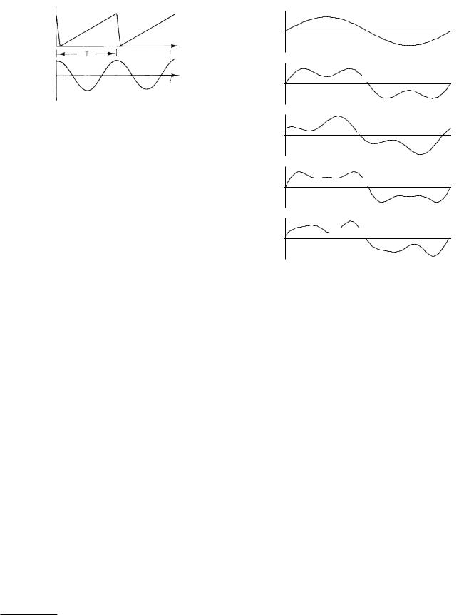
FIGURE 11.3. Two di erent periodic functions.

Since y and its derivatives can be evaluated using the current guess for each b, the expression is linear in the hk, and the linear least-squares technique can be used to determine the values of the hk that minimize Q. After each hk has been determined, the revised values bk = bk0 + hk are used as the initial guesses, and the process is repeated until a minimum value of Q is found. The technique is not always stable; it can overshoot and give too large a value for hk . There are many ways to improve the process to ensure more rapid convergence. The most common is called the Levenberg–Marquardt method [see Bevington and Robinson (1992) or Press et al. (1992)].

11.3The Presence of Many Frequencies in a Periodic Function

A function y that repeats itself after a time2 T is said to be periodic with period T . The mathematical description of this periodicity is

Two examples of functions with period T are shown in Fig. 11.3. One of these functions is a sine wave, y(t) = A sin(ω0t−φ), where A is the amplitude, ω0 is the angular frequency, and φ is the phase of the function. Changing the amplitude changes the height of the function. Changing the phase shifts the function along the time axis. The sine function repeats itself when the argument shifts by 2π radians. It repeats itself after time T , where ω0T = 2π. Therefore the angular frequency is related to the period by

(The units of ω0 are radian s−1, but radians are dimensionless.) It is completely equivalent to write the function in terms of the frequency as y(t) = A sin (2πf0t −φ). The

2Although we speak of t and time, the technique can be applied to any independent variable if the dependent variable repeats as in Eq. 11.10. Zebra stripes are (almost) periodic functions of position.

FIGURE 11.4. Various periodic signals made by adding sine waves that are harmonically related. Each signal has an angular frequency ω0 = 1 and a period T = 2π.

frequency f0 is the number of cycles per second. Its units are s−1 or hertz (Hz) (hertz is not used for angular frequency):

It is possible to write function y as a sum of a sine term and a cosine term instead of using phase φ:

y(t) = A sin(ω0t − φ) = A(sin ω0t cos φ − cos ω0t sin φ)

The upper function graphed in Fig. 11.3 also has period

T .

Harmonics are integer multiples of the fundamental frequency. They have the time dependence cos(kω0t) or sin(kω0t), where k = 2, 3, 4, . . . . These also have period T . (They also have shorter periods, but they still satisfy the definition Eq. 11.10 for a function of period T .)

We can generate periodic functions of di erent shapes by combining various harmonics. Di erent combinations of the fundamental, third harmonic, and fifth harmonic are shown in Fig. 11.4. In this figure, (a) is a pure sine wave, (b) and (c) have some third harmonic added with a di erent phase in each case, and (d) and (e) show the addition of a fifth harmonic term to (b) with di erent phases.

290 11. The Method of Least Squares and Signal Analysis

An even function is one for which y(t) = y(−t). For an odd function, y(t) = −y(−t). The cosine is even, and the sine is odd. A sum of sine terms gives an odd function. A sum of cosine terms gives an even function.

−bk sin(kω0tj ) cos(mω0tj ) ,

k=1

11.4 Fourier Series for Discrete Data

11.4.1 Introducing the Fourier Series

The ability to adjust the amplitude of sines and cosines to approximate a specific shape suggests that discrete periodic data can be fitted by a function of the form

(11.14)

It is important to note that if we have a set of data to fit, in some cases we may not know the actual period of the data; we sample for some interval of length T . In that case the period T = 2π/ω0 is a characteristic of the fitting function that we calculate, not of the data being fitted.

There are 2n + 1 parameters (a0; a1, . . . , an; b1, . . . , bn). Since there are N independent data points, there can be at most N independent coe cients. Therefore, 2n + 1 ≤ N , or

This means that there must be at least two samples per period at the highest frequency present. This is known as the Nyquist sampling criterion.

If the least-squares criterion is used to determine the parameters, Eq. 11.14 is a Fourier-series representation of the data. Using the least-squares criterion to determine the coe cients to fit N data points requires minimizing the mean square residual

k=1

The derivatives that must be set to zero are

−bk sin(kω0tj ) (1) ,

k=1

and

−bk sin(kω0tj ) sin(mω0tj ) .

k=1

Setting each derivative equal to zero and interchanging the order of the summations give 2n + 1 equations analogous to Eq. 11.8. The first is

nN

+bk sin(kω0tj ).

k=1 j=1

There are n equations of the form

nN

+ak cos(kω0tj ) cos(mω0tj )

k=1 j=1

(11.18)

nN

+bk sin(kω0tj ) cos(mω0tj )

k=1 j=1

for m = 1, . . . , n, and n more of the form

nN

+ak cos(kω0tj ) sin(mω0tj )

k=1 j=1

nN

+bk sin(kω0tj ) sin(mω0tj ).

k=1 j=1

(11.19)

Since the tj are known, each of the sums over the data points (index j) on the right-hand side can be evaluated independent of the yj .

11.4.2Equally Spaced Data Points Simplify the Equations

If the data points are equally spaced, the equations become much simpler. There are N data points spread out

over an interval T : tj = jT /N = 2πj/N ω0, j = 1, . . . , N . The arguments of the sines and cosines are of the form (2πjk/N ). One can show that

j=1

Because of these properties, Eqs. 11.17–11.19 become a set of independent equations when the data are equally spaced:

11.4.3The Standard Form for the Discrete Fourier Transform

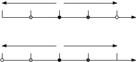
It is customary to change the notation to make the equations more symmetric. Figure 11.5 shows the four different times corresponding to N = 4 with j = 1, 2, 3, 4. Because of the periodicity of the sines and cosines, j = N gives exactly the same value of a sine or cosine as does j = 0. Therefore, if we reassign the data point corresponding to j = N to have the value j = 0 and sum from 0 to N − 1, the sums will be unchanged:

FIGURE 11.5. A case where N = 4. The values of time are spaced by T /N and distributed uniformly. In the top case the values of j range from 1 to N . In the lower case they range from 0 to N −1. The values of all the trigonometric functions are the same for j = 0 and for j = N .

For equally spaced data the function can be written as

(11.26d) You can show (see the problems at the end of this chapter) that the symmetry and antisymmetry in Eqs. 11.22 and 11.23 for k = N −m means that Eqs. 11.25 and 11.26 for k > N/2 repeat those for k < N/2. We can use this fact to make the equations more symmetric by changing the factor in front of the summations in Eqs. 11.26b and 11.26c to be 1/N instead of 2/N and extending the summation in Eq. 11.26d all the way to n = N − 1. Since cos(0) = 1 and sin(0) = 0, we can include the term a0 by including k = 0 in the sum. We then have the set of

equations

This set of equations is the usual form for the discrete Fourier transform. We will continue to use our earlier form, Eqs. 11.26, in the rest of this chapter.

11.4.4Complex Exponential Notation

The Fourier transform is usually written in terms of complex exponentials. We have avoided using complex exponentials. They are not necessary for anything done in this

R2

Q = 0.1907

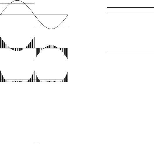
FIGURE 11.6. A square wave y(tj ) and the calculated function y(t) = b1 sin(ω0t) are shown, along with the residuals and the squares of the residuals for each point. The value of b1 is 4/π, which minimizes Q for that term.

book. The sole advantage of complex exponentials is to simplify the notation. The actual calculations must be done with real numbers. Since you will undoubtedly see complex notation in other books, the notation is included here for completeness.

The numbers that we have been using are called real

√

numbers. The number i = −1 is called an imaginary number. A combination of a real and imaginary number is called a complex number. The remarkable property of imaginary numbers that make them useful in this context is that

If we define the complex number Yk = ak − ibk , we can write Eqs. 11.27 as

k=0

Since our function y is assumed to be real, in the second equation we keep only the real part of the sum. To repeat: this gives only a more compact notation. It does not save in the actual calculations.

11.4.5 Example: The Square Wave

Figures 11.6–11.9 show fits to a square wave with 128 data points. The function is yj = 1, j = 0, . . . , 63 and yj = −1,

j = 64, . . . , 127. This is an odd function of t. Therefore, the series should contain only sine terms; all ak should be zero. The calculated coe cients are shown in Table 11.3. Some of the ak values are small but not exactly zero. This is due to the finite number of data points; the ak become smaller as N is increased. The even values of the bk vanish. We will see why below.

Figure 11.6 shows the square wave as dots and y(x) as a smooth curve when b1 = 1.273 and all the other coe - cients are zero. This provides the minimum Q obtainable with a single term. Figure 11.7 shows why Q is larger for any other value of b1. Figure 11.8 shows the terms for k = 1 and k = 3. The value of Q is further reduced. Figure 11.9 shows why even terms do not reduce Q. In this case b2 = 0.5 has been added to b1. The fit is improved for the regions 0 < t < T /4 and 3T /4 < t < T , but between those regions the fit is made worse.

11.4.6Example: When the Sampling Time Is Not a Multiple of the Period of the Signal

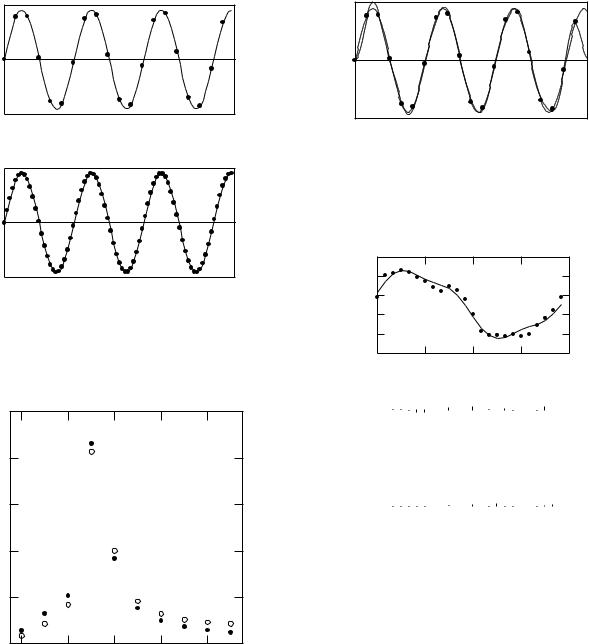
The discussion just after Eq. 11.14 pointed out that in some cases we may not know the actual period and fundamental frequency ω0 of the data. If we do know the actual period and the data points yj are a sine or cosine with exact frequency ω0 or a harmonic, and if no random errors are superimposed on the data, then only the coe - cients corresponding to those frequencies will be nonzero. The reason is that if the function is exactly periodic, then by sampling for one period we have e ectively sampled for an infinite time.

If the measuring duration T is not an integral multiple of the period of the signal—that is, the frequency of the signal y is not an exact harmonic of ω0—then the Fourier series contains terms at several frequencies.

N = 20 and N = 80 samples during the period of the measurement. For 20 samples, n = 9; for 80 samples, n = 39. Figure 11.11 shows (a2k + b2k )1/2 for both sample sets for k = 0 to 9, calculated using Eqs. 11.26. For

FIGURE 11.7. A single term is used to approximate the square wave. (a) b1 = 1.00, which is too small a value. (b) b1 = 1.75, which is too large. In both cases Q is larger than the minimum value for a single term, shown in Fig. 11.6.

80 samples, the value of (a2k + b2k )1/2 is very small for k > 9 and is not plotted. The frequency spectrum is virtually independent of the number of samples. There is a zero-frequency component because there is a net positive area under the curve. The largest amplitude occurs for k = 3. If one imagines a smooth curve drawn through the histogram, its peak would be slightly above k = 3. We will see later that the width of this curve depends on the duration of the measurement, T .

Figure 11.12 shows the fit to the data of Fig. 11.10a. Since the data points had no errors, the fitting function with 20 parameters passes through each of the 20 data points. However, it does not match y of Fig. 11.10a at

FIGURE 11.9. This figure shows why even terms do not contribute. A term b2 = 0.5 has been added to a term with the correct value of b1. It improves the fit for t < T /4 and t > 3T /4 but makes it worse between T /4 and 3T /4.

other points. Note particularly the di erence between the function near j = 1 and near j = 19.

11.4.7 Example: Spontaneous Births

Figure 11.13 shows the number of spontaneous births per hour vs. local time of day for 600,000 live births in various parts of the world. The basic period is 24 hr; there is also a component with k = 3 (T = 8 hr). These data were reported by Kaiser and Halberg (1962). More recent data show peaks at di erent times [Anderka et al. (2000)]. Changes might be due to a di erence in the duration of labor.

FIGURE 11.10. Sine wave yj = sin [3.3 × 2πj/N ] (a) with 20 data points and (b) with 80 data points. The sampling time is not an integral number of periods.

0.2N = 80

N = 20

0.0

k

FIGURE 11.11. The amplitude of the mixed sine and cosine coe cients (a2k + b2k )1/2 vs k for the function yj = sin 3.3 × 2πj/N . The signal is sampled for 20 (open circles) or 80 (solid circles) data points. The amplitude spectrum is nearly independent of the number of samples.

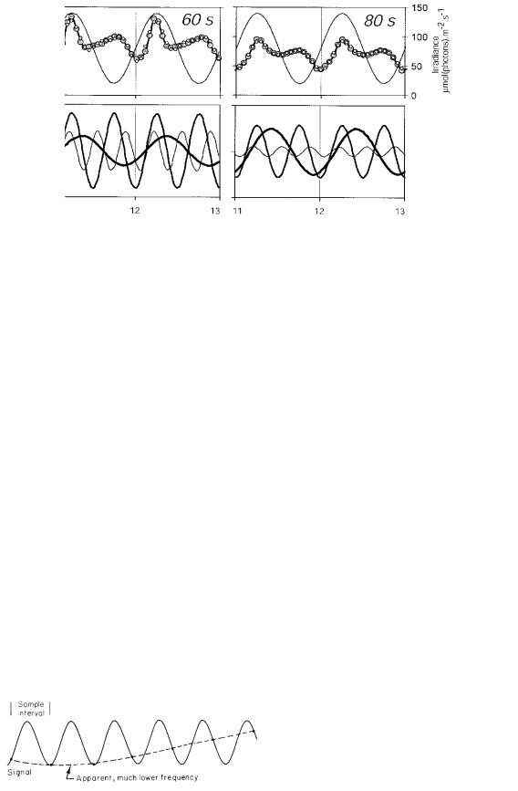
11.4.8 Example: Photosynthesis in Plants

Tobacco plant leaves were exposed to white light similar to sunlight, with the amplitude varying sinusoidally with a frequency ω0 corresponding to a period of 60 or 80 s [Nedbal and Bˇrezina (2002)]. Fluorescence measurements showed an oscillation with predominant frequencies of ω0,

FIGURE 11.12. The solid line shows the calculated fit for the 20 data points in Fig. 11.10a. The dashed line is the same as the solid line in Fig. 11.10.

FIGURE 11.13. Data on the number of spontaneous births per hour, fit with terms having a period of 24 hr and 8 hr.

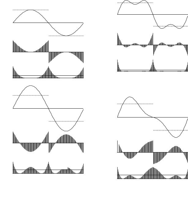
2ω0, and 3ω0. This is shown in Fig. 11.14. The authors present a feedback model, very similar to those in Sections 10.10.6 and 11.15. A nonlinearity in the model is responsible for generating the second and third harmonics.

11.4.9Pitfalls of Discrete Sampling: Aliasing

We saw in the preceding section that N samples in time T allow the determination of unique Fourier coe cients only for the terms from k = 0 to n = (N − 1)/2. This means that for a sampling interval T /N , the maximum angular frequency is (N − 1)ω0/2. The period of the highest frequency that can be determined is Tmin = 2T /(N −1). This is approximately twice the spacing of the data points. One must sample at least twice per period to determine the coe cient at a particular frequency.

If a component is present whose frequency is more than half the sampling frequency, it will appear in the analysis at a lower frequency. This is the familiar stroboscopic e ect in which the wheels of the stagecoach appear to rotate backward because the samples (movie frames) are not made rapidly enough. In signal analysis, this is called aliasing. It can be seen in Fig. 11.15, which shows a sine wave sampled at regularly spaced intervals that are longer than half a period.

This phenomenon is inescapable if frequencies greater than (N − 1)ω0/2 are present. They must be removed by analog or digital techniques before the sampling is done. For a more detailed discussion, see Blackman and Tukey (1958) or Press et al. (1992). An example of aliasing is found in a later section, in Fig. 11.41. Maughan et al. (1973) pointed out how researchers have been “stung” by this problem in hematology.

of the sines and cosines, which uses a lot of computer time. Cooley and Tukey (1965) showed that it is possible to group the data in such a way that the number of multiplications is about (N/2) log2 N instead of N 2 and the sines and cosines need to be evaluated only once, a technique known as the Fast Fourier Transform (FFT). For example, for 1024 = 210 data points, N 2 = 1 048 576, while (N/2) log2 N = (512)(10) = 5120. This speeds up the calculation by a factor of 204. The techniques for the FFT are discussed by many authors [see Press et al. (1992) or Visscher (1996)]. Bracewell (1990) has written an interesting review of all the popular numerical transforms. He points out that the grouping used in the FFT dates back to Gauss in the early nineteenth century.

11.4.10Fast Fourier Transform

The calculation of the Fourier coe cients using our equations involves N evaluations of the sine or cosine, N multiplications, and N additions for each coe cient. There are N coe cients, so that there must be N 2 evaluations

FIGURE 11.15. An example of aliasing. The data are sampled less often than twice per period and appear to be at a much lower frequency.

11.5Fourier Series for a Periodic Function

It is possible to define the Fourier series for a continuous periodic function y(t) as well as for discrete data points yj . In fact, the function need only be piecewise continuous, that is, with a finite number of discontinuities. The calculated function is given by the analog of Eq. 11.14:

The quantity to be minimized is still the mean square error, in this case

y(t) − a0 − [ak cos(kω0t) + bk sin(kω0t)]

k=1

× cos(mω0t) dt = 0.

This integral must be zero for each value of m from 1 to n. If the order of integration and summation is interchanged, the result is

−ak cos(kω0t) cos(mω0t) dt

k=1 0

nT

− bk sin(kω0t) cos(mω0t) dt = 0.

k=1 0

The integral of cos(mω0t) over a period vanishes. The last two integrals are of the form given in Appendix E, Eqs. E.4 and E.5:

sin(kω0t) cos(mω0t) dt = 0.

0

(11.32) These results are the orthogonality relations for the trigonometric functions. Inserting these values, we find that only one term in the first summation over k remains, and we have

These equations are completely general. Because of the orthogonality of the integrals, the coe cients are independent, just as they were in the discrete case for equally spaced data. This is not surprising, since the continuous case corresponds to an infinite set of uniformly spaced data.

Note the similarity of these equations to the discrete results, Eqs. 11.25. In each case a0 is the average of the function over the period. The other coe cients are twice the average of the signal multiplied by the sine or cosine whose coe cient is being calculated.

The integrals can be taken over any period. Sometimes it is convenient to make the interval −T /2 to T /2. As we would expect, the integrals involving sines vanish when y is an even function, and those involving cosines vanish when y is an odd function.

For the square wave y(t) = 1, 0 < t < T /2; y(t) = −1, T /2 < t < T , we find

Table 11.4 shows the first few coe cients for the Fourier series representing the square wave, obtained from Eq. 11.34. They are the same as those for the discrete data in Table 11.3. Figure 11.16 shows the fits for n = 3 and n = 39. As the number of terms in the fit is increased, the value of Q decreases. However, spikes of constant height (about 18% of the amplitude of the square wave or 9% of the discontinuity in y) remain. These are seen in Fig. 11.16. These spikes appear whenever there is a discontinuity in y and are called the Gibbs phenomenon.

Figure 11.17 shows the blood flow in the pulmonary artery of a dog as a function of time. It has been fitted by a mean and four terms of the form Mk sin(kω0t −φk). The technique is useful because the elastic properties of the arterial wall can be described in terms of sinusoidal pressure variations at various frequencies [Milnor (1972)].