

60 |
Mathematics |
|
|
2.14Numerical methods
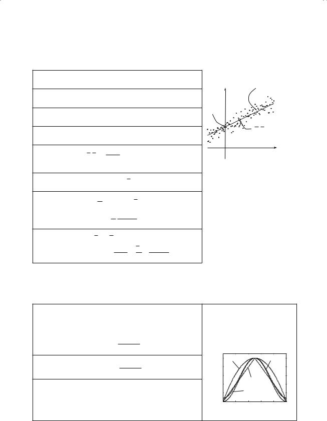
Straight-line fittinga
Data |
{xi},{yi} |
|
n points |
|
(2.570) |
y |
y = mx+ c |
|||||||||||
|
|
|
|
|
|
|
|
|
|
|
|
|
|
|
|
|
|
|
Weightsb |
{wi} |
|
|
|
|
|
|
|
|
|
|
|
|
|
(2.571) |
|
|
|
|
y = mx+ c |
|
|
|
|
|
|
|
|
|
(2.572) |
(0,c) |
|
|||||
Model |
|
|
|
|
|
|
|
|
|
|
|
|||||||
Residuals |
di = yi − mxi − c |
|
|
|
|
|
(2.573) |
|
(x,y) |
|||||||||
|
|
|
|
|
|
|
||||||||||||
|
|
|
|
|
|
1 |
|
|
wixi , |
wiyi! |
|
|
x |
|||||
Weighted |
|
|
|
|
|
|
|
|
|
|
||||||||
(x,y) = wi |
|
|
|
|
||||||||||||||
centre |
|
(2.574) |
|
|
||||||||||||||
Weighted |
D = wi(xi − x)2 |
|
|
|
(2.575) |
|
|
|||||||||||
moment |
|
|
|
|
|
|||||||||||||
Gradient |
m |
= |
1 |
|
|
i |
( |
x |
i |
− |
2 ) |
y |
i |
|
(2.576) |
|
|
|
D |
|
|
|
|
||||||||||||||
|
|
|
|
|
w |
|
|
|
|
x |
|
|
|
|
|
|||
|
var[m] |
|
1 |
|
|
widi |
|
|
|
(2.577) |
|
|
||||||
|
D − 2 |
|
|
|
|
|
|
|||||||||||
|
|
|
|
|
|
|
|
n |
|
|
|
|
|
|
|
|
|
|
|
c = y − mx |
|
|
|
i |
|
|
|
− 2 |
(2.578) |
|
|
||||||
a |
|
|
|
|
|
|
|
|
|
|
|
|
|
|
||||
Intercept |
var[c] |
|
|
|
1 |
|
|
x2 |
|
widi2 |
(2.579) |
|
|
|||||
|
|
|
|
|
w |
|
+ D |
|
n |
|
|
|||||||
bLeast-squares fit of data to |
y |
|
|
mx+ c. Errors on y-values only. |
|
|
||||||||||||
|
= |
|
|
|
|
|
|
|
|
|
|
|
||||||
If the errors on yi are uncorrelated, then wi = 1/var[yi]. |
|
|
|
|||||||||||||||
Time series analysisa
Discrete |
|
|
|
|
|
M/2 |
|
|
|
|
||
(r s)j = |
k=−( 2)+1 |
sj−krk |
(2.580) |
|||||||||
convolution |
||||||||||||
|
|
|
|
|
|
M/ |
|
|
|
|
||
|
|
|
|
|
|
|
|
|
|
|
|
|
Bartlett |
|
|
|
|
|
|
|
|
|
|
|
|
|
|
|
|
|
|
|
|
|
|
|||
(triangular) |
wj = 1 |
− |
|
j − N/2 |
|
|
|
(2.581) |
||||
window |
|
|
|
N/2 |
|
|
|
|||||
Welch |
|
|
|
|
|
|
|
|
|
2 |
|
|
|
|
|
j |
|
N/2 |
|
|
|
||||
(quadratic) |
wj = 1 |
− |
|
|
− |
|
|
|
(2.582) |
|||
window |
|
|
N/2 |
|
|
|||||||
Hanning |
wj = |
1 |
1 − cos |
2πj |
|
|
(2.583) |
|
window |
|
|
|
|
|
|||
2 |
N |
|
|
|||||
Hamming |
wj = 0.54 − 0.46cos |
2πj |
|
(2.584) |
||||
window |
|
|||||||
N |
||||||||
ri |
response function |
si |
time series |
Mresponse function duration
wj windowing function
Nlength of time series
1 |
Welch |
Hamming |
0.8 |
|
|
w 0.6 |
|
Bartlett |
0.4 |
|
|
|
|
|
0.2 |
|
Hanning |
|
|
|
0 |
|
|
0 |
0.2 0.4 0.6 0.8 1 |
|
|
|
j/N |
aThe time series runs from j = 0...(N − 1), and the windowing functions peak at j = N/2.
2.14 Numerical methods |
61 |
|
|
Numerical integration
|
|
h |
|
|
|
|
2 |
|
|
|
|
f(x) |
|
|
|
|
|
|
|
|
|
|
|
|
|
|
|
x |
|
|
|
|
x0 |
|
|
xN |
|
|
|
|
xN |
|
h |
|
|
h |
= (xN − x0)/N |
|
x0 |
f(x) dx |
(f0 + 2f1 + 2f2 + · · · |
|
|
(subinterval |
|
Trapezoidal rule |
2 |
|
fi |
width) |
|||
|
|
|
|
+ 2fN−1 + fN ) |
(2.585) |
fi = f(xi) |
|
|
|
|
|
N |
number of |
||
|
|
|
|
|
|
|
subintervals |
|
xN |
|
h |
|
|
|
|
|
x0 |
f(x) dx |
(f0 + 4f1 + 2f2 + 4f3 |
+ · · · |
|
|
|
Simpson’s rulea |
3 |
|
|
||||
|
|
|
|
+ 4fN−1 + fN ) |
(2.586) |
|
|
aN must be even. Simpson’s rule is exact for quadratics and cubics. |
|
|
|
||||
Numerical di erentiationa
|
df |
|
|
1 |
|
|
|
|
|
|
||
|
|
|
|
|
|
|
[−f(x+ 2h) + 8f(x+ h) − 8f(x− h) + f(x− 2h)] |
(2.587) |
||||
|
dx |
12h |
||||||||||
|
|
|
|
1 |
[f(x+ h) − f(x− h)] |
(2.588) |
||||||
|
|
|
|
|||||||||
|
|
2h |
||||||||||
|
|
|
|
|
|
|
|
|
|
|||
|
d2f |
|
1 |
|
[−f(x+ 2h) + 16f(x+ h) − 30f(x) + 16f(x− h) − f(x− 2h)] |
(2.589) |
||||||
|
dx2 |
|
12h2 |
|||||||||
|
|
|
|
|
1 |
|
|
|
|
|
||
|
|
|
|
|
[f(x+ h) − 2f(x) + f(x− h)] |
(2.590) |
||||||
|
|
|
h2 |
|||||||||
|
d3f |
|
1 |
|
[f(x+ 2h) − 2f(x+ h) + 2f(x− h) − f(x− 2h)] |
(2.591) |
||||||
|
dx3 |
|
2h3 |
|||||||||
aDerivatives of f(x) at x. h is a small interval in x.
Relations containing “ ” are O(h4); those containing “ ” are O(h2).
Numerical solutions to f(x) = 0
Secant method |
xn+1 = xn |
|
xn − xn−1 |
f(xn) (2.592) |
f |
function of x |
||
|
|
f(x∞ ) = 0 |
||||||
|
|
− f(xn) − f(xn−1) |
|
xn |
||||
Newton–Raphson |
xn+1 = xn |
|
f(xn) |
|
(2.593) |
f |
= df/dx |
|
method |
− f (xn) |
|||||||
|
|
|
|
|||||

62 Mathematics
Numerical solutions to ordinary di erential equationsa
|
if |
|
dy |
|
= f(x,y) |
(2.594) |
|
|
dx |
||||
|
|
|
|
|
||
Euler’s method |
and |
|
h = xn+1 − xn |
(2.595) |
||
|
|
|||||
|
then |
yn+1 |
= yn + hf(xn,yn) + O(h2) |
(2.596) |
||
Runge–Kutta method (fourth-order)
if |
|
dy |
|
= f(x,y) |
|
|
|
|
|
|
|
(2.597) |
||
|
dx |
|
|
|
|
|
|
|
||||||
|
|
|
|
|
|
|
|
|
|
|
|
|
||
and |
|
h = xn+1 − xn |
|
|
|
|
|
|
|
(2.598) |
||||
|
|
k1 |
= hf(xn,yn) |
|
|
|
|
|
|
|
(2.599) |
|||
|
|
k2 |
= hf(xn + h/2,yn + k1/2) |
|
(2.600) |
|||||||||
|
|
k3 |
= hf(xn + h/2,yn + k2/2) |
|
(2.601) |
|||||||||
|
|
k4 |
= hf(xn + h,yn + k3) |
|
|
|
(2.602) |
|||||||
|
|
|
|
k1 |
k2 |
k3 |
k4 |
+ O(h5) |
|
|||||
then |
yn+1 |
= yn + |
|
+ |
|
+ |
|
+ |
|
|
(2.603) |
|||
6 |
3 |
3 |
6 |
|
||||||||||
aOrdinary di erential equations (ODEs) of the form ddxy = f(x,y). Higher order equations should be reduced to a set of coupled first-order equations and solved in parallel.