

- •List of Tables
- •List of Figures
- •Table of Notation
- •Preface
- •Boolean retrieval
- •An example information retrieval problem
- •Processing Boolean queries
- •The extended Boolean model versus ranked retrieval
- •References and further reading
- •The term vocabulary and postings lists
- •Document delineation and character sequence decoding
- •Obtaining the character sequence in a document
- •Choosing a document unit
- •Determining the vocabulary of terms
- •Tokenization
- •Dropping common terms: stop words
- •Normalization (equivalence classing of terms)
- •Stemming and lemmatization
- •Faster postings list intersection via skip pointers
- •Positional postings and phrase queries
- •Biword indexes
- •Positional indexes
- •Combination schemes
- •References and further reading
- •Dictionaries and tolerant retrieval
- •Search structures for dictionaries
- •Wildcard queries
- •General wildcard queries
- •Spelling correction
- •Implementing spelling correction
- •Forms of spelling correction
- •Edit distance
- •Context sensitive spelling correction
- •Phonetic correction
- •References and further reading
- •Index construction
- •Hardware basics
- •Blocked sort-based indexing
- •Single-pass in-memory indexing
- •Distributed indexing
- •Dynamic indexing
- •Other types of indexes
- •References and further reading
- •Index compression
- •Statistical properties of terms in information retrieval
- •Dictionary compression
- •Dictionary as a string
- •Blocked storage
- •Variable byte codes
- •References and further reading
- •Scoring, term weighting and the vector space model
- •Parametric and zone indexes
- •Weighted zone scoring
- •Learning weights
- •The optimal weight g
- •Term frequency and weighting
- •Inverse document frequency
- •The vector space model for scoring
- •Dot products
- •Queries as vectors
- •Computing vector scores
- •Sublinear tf scaling
- •Maximum tf normalization
- •Document and query weighting schemes
- •Pivoted normalized document length
- •References and further reading
- •Computing scores in a complete search system
- •Index elimination
- •Champion lists
- •Static quality scores and ordering
- •Impact ordering
- •Cluster pruning
- •Components of an information retrieval system
- •Tiered indexes
- •Designing parsing and scoring functions
- •Putting it all together
- •Vector space scoring and query operator interaction
- •References and further reading
- •Evaluation in information retrieval
- •Information retrieval system evaluation
- •Standard test collections
- •Evaluation of unranked retrieval sets
- •Evaluation of ranked retrieval results
- •Assessing relevance
- •A broader perspective: System quality and user utility
- •System issues
- •User utility
- •Results snippets
- •References and further reading
- •Relevance feedback and query expansion
- •Relevance feedback and pseudo relevance feedback
- •The Rocchio algorithm for relevance feedback
- •Probabilistic relevance feedback
- •When does relevance feedback work?
- •Relevance feedback on the web
- •Evaluation of relevance feedback strategies
- •Pseudo relevance feedback
- •Indirect relevance feedback
- •Summary
- •Global methods for query reformulation
- •Vocabulary tools for query reformulation
- •Query expansion
- •Automatic thesaurus generation
- •References and further reading
- •XML retrieval
- •Basic XML concepts
- •Challenges in XML retrieval
- •A vector space model for XML retrieval
- •Evaluation of XML retrieval
- •References and further reading
- •Exercises
- •Probabilistic information retrieval
- •Review of basic probability theory
- •The Probability Ranking Principle
- •The 1/0 loss case
- •The PRP with retrieval costs
- •The Binary Independence Model
- •Deriving a ranking function for query terms
- •Probability estimates in theory
- •Probability estimates in practice
- •Probabilistic approaches to relevance feedback
- •An appraisal and some extensions
- •An appraisal of probabilistic models
- •Bayesian network approaches to IR
- •References and further reading
- •Language models for information retrieval
- •Language models
- •Finite automata and language models
- •Types of language models
- •Multinomial distributions over words
- •The query likelihood model
- •Using query likelihood language models in IR
- •Estimating the query generation probability
- •Language modeling versus other approaches in IR
- •Extended language modeling approaches
- •References and further reading
- •Relation to multinomial unigram language model
- •The Bernoulli model
- •Properties of Naive Bayes
- •A variant of the multinomial model
- •Feature selection
- •Mutual information
- •Comparison of feature selection methods
- •References and further reading
- •Document representations and measures of relatedness in vector spaces
- •k nearest neighbor
- •Time complexity and optimality of kNN
- •The bias-variance tradeoff
- •References and further reading
- •Exercises
- •Support vector machines and machine learning on documents
- •Support vector machines: The linearly separable case
- •Extensions to the SVM model
- •Multiclass SVMs
- •Nonlinear SVMs
- •Experimental results
- •Machine learning methods in ad hoc information retrieval
- •Result ranking by machine learning
- •References and further reading
- •Flat clustering
- •Clustering in information retrieval
- •Problem statement
- •Evaluation of clustering
- •Cluster cardinality in K-means
- •Model-based clustering
- •References and further reading
- •Exercises
- •Hierarchical clustering
- •Hierarchical agglomerative clustering
- •Time complexity of HAC
- •Group-average agglomerative clustering
- •Centroid clustering
- •Optimality of HAC
- •Divisive clustering
- •Cluster labeling
- •Implementation notes
- •References and further reading
- •Exercises
- •Matrix decompositions and latent semantic indexing
- •Linear algebra review
- •Matrix decompositions
- •Term-document matrices and singular value decompositions
- •Low-rank approximations
- •Latent semantic indexing
- •References and further reading
- •Web search basics
- •Background and history
- •Web characteristics
- •The web graph
- •Spam
- •Advertising as the economic model
- •The search user experience
- •User query needs
- •Index size and estimation
- •Near-duplicates and shingling
- •References and further reading
- •Web crawling and indexes
- •Overview
- •Crawling
- •Crawler architecture
- •DNS resolution
- •The URL frontier
- •Distributing indexes
- •Connectivity servers
- •References and further reading
- •Link analysis
- •The Web as a graph
- •Anchor text and the web graph
- •PageRank
- •Markov chains
- •The PageRank computation
- •Hubs and Authorities
- •Choosing the subset of the Web
- •References and further reading
- •Bibliography
- •Author Index
14.1 Document representations and measures of relatedness in vector spaces
x2 x3 x4
|
|
dtrue |
x′ |
x′ |
|
x′ |
x |
1 |
x5 |
x3′ |
|||
|
|
1 |
2 |
4 |
291
x5′
x1′ |
x2′ x3′ x4′ |
x5′ |
||
|
dprojected |
|
|
|
|
|
|
||
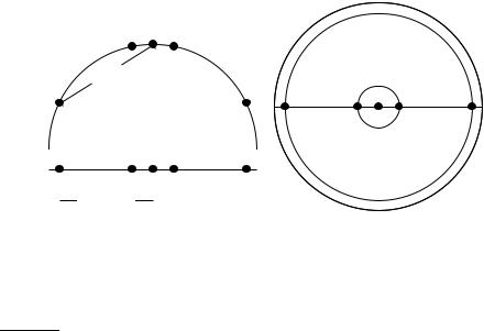
Figure 14.2 Projections of small areas of the unit sphere preserve distances. Left: A projection of the 2D semicircle to 1D. For the points x1, x2, x3, x4, x5 at x coordinates −0.9, −0.2, 0, 0.2, 0.9 the distance |x2x3| ≈ 0.201 only differs by 0.5% from |x2′ x3′ | =
0.2; but |x1x3|/|x1′ x3′ | = dtrue/dprojected ≈ 1.06/0.9 ≈ 1.18 is an example of a large distortion (18%) when projecting a large area. Right: The corresponding projection of
the 3D hemisphere to 2D.
are not systematically better than linear models. Nonlinear models have more parameters to fit on a limited amount of training data and are more likely to make mistakes for small and noisy data sets.
When applying two-class classifiers to problems with more than two classes, there are one-of tasks – a document must be assigned to exactly one of several mutually exclusive classes – and any-of tasks – a document can be assigned to any number of classes as we will explain in Section 14.5. Two-class classifiers solve any-of problems and can be combined to solve one-of problems.
14.1Document representations and measures of relatedness in vector spaces
As in Chapter 6, we represent documents as vectors in R|V| in this chapter. To illustrate properties of document vectors in vector classification, we will render these vectors as points in a plane as in the example in Figure 14.1. In reality, document vectors are length-normalized unit vectors that point to the surface of a hypersphere. We can view the 2D planes in our figures as projections onto a plane of the surface of a (hyper-)sphere as shown in Figure 14.2. Distances on the surface of the sphere and on the projection plane are approximately the same as long as we restrict ourselves to small areas of the surface and choose an appropriate projection (Exercise 14.1).
Online edition (c) 2009 Cambridge UP

292 |
14 Vector space classification |
Decisions of many vector space classifiers are based on a notion of distance, e.g., when computing the nearest neighbors in kNN classification. We will use Euclidean distance in this chapter as the underlying distance measure. We observed earlier (Exercise 6.18, page 131) that there is a direct correspondence between cosine similarity and Euclidean distance for lengthnormalized vectors. In vector space classification, it rarely matters whether the relatedness of two documents is expressed in terms of similarity or distance.
However, in addition to documents, centroids or averages of vectors also play an important role in vector space classification. Centroids are not lengthnormalized. For unnormalized vectors, dot product, cosine similarity and Euclidean distance all have different behavior in general (Exercise 14.6). We will be mostly concerned with small local regions when computing the similarity between a document and a centroid, and the smaller the region the more similar the behavior of the three measures is.
?Exercise 14.1
For small areas, distances on the surface of the hypersphere are approximated well by distances on its projection (Figure 14.2) because α ≈ sin α for small angles. For what size angle is the distortion α/ sin(α) (i) 1.01, (ii) 1.05 and (iii) 1.1?
14.2Rocchio classification
DECISION BOUNDARY
ROCCHIO CLASSIFICATION CENTROID
(14.1)
Figure 14.1 shows three classes, China, UK and Kenya, in a two-dimensional (2D) space. Documents are shown as circles, diamonds and X’s. The boundaries in the figure, which we call decision boundaries, are chosen to separate the three classes, but are otherwise arbitrary. To classify a new document, depicted as a star in the figure, we determine the region it occurs in and assign it the class of that region – China in this case. Our task in vector space classification is to devise algorithms that compute good boundaries where “good” means high classification accuracy on data unseen during training.
Perhaps the best-known way of computing good class boundaries is Rocchio classification, which uses centroids to define the boundaries. The centroid of a class c is computed as the vector average or center of mass of its members:
1
~µ(c) = |Dc| d∑Dc ~v(d)
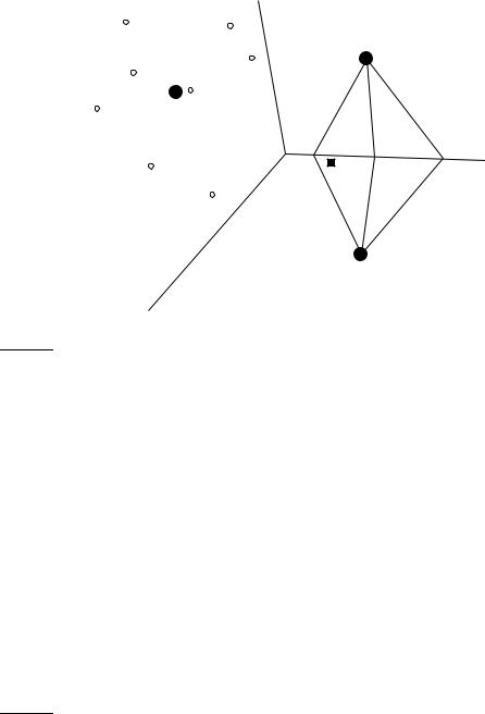
where Dc is the set of documents in D whose class is c: Dc = {d : hd, ci D}. We denote the normalized vector of d by ~v(d) (Equation (6.11), page 122). Three example centroids are shown as solid circles in Figure 14.3.
The boundary between two classes in Rocchio classification is the set of points with equal distance from the two centroids. For example, |a1| = |a2|,
Online edition (c) 2009 Cambridge UP
14.2 Rocchio classification |
|
|
|
293 |
|
|
|
|
|
|
|
|
|
|
|
|
|
|
|
|
|
|
|
|
|
|
|
|
UK |
a1 |
|
b1 |
c1 |
|
|
|
|||
|
|
|
|
|
|
a2 |
|
b2 |
c2 |
China
x |
x |
|
x |
||
|
||
Kenya |
x |
|
|
Figure 14.3 Rocchio classification.
|b1| = |b2|, and |c1| = |c2| in the figure. This set of points is always a line. The generalization of a line in M-dimensional space is a hyperplane, which we define as the set of points ~x that satisfy:
(14.2) w~ T~x = b
NORMAL VECTOR where w~ is the M-dimensional normal vector1 of the hyperplane and b is a constant. This definition of hyperplanes includes lines (any line in 2D can be defined by w1x1 + w2x2 = b) and 2-dimensional planes (any plane in 3D can be defined by w1x1 + w2x2 + w3x3 = b). A line divides a plane in two, a plane divides 3-dimensional space in two, and hyperplanes divide higherdimensional spaces in two.
Thus, the boundaries of class regions in Rocchio classification are hyperplanes. The classification rule in Rocchio is to classify a point in accordance with the region it falls into. Equivalently, we determine the centroid ~µ(c) that the point is closest to and then assign it to c. As an example, consider the star in Figure 14.3. It is located in the China region of the space and Rocchio therefore assigns it to China. We show the Rocchio algorithm in pseudocode in Figure 14.4.
1. Recall from basic linear algebra that ~v · w~ = ~vT w~ , i.e., the dot product of ~v and w~ equals the product by matrix multiplication of the transpose of ~v and w~ .
Online edition (c) 2009 Cambridge UP
294 |
|
|
|
|
|
|
|
14 Vector space classification |
||
|
vector |
|
|
term weights |
|
|
|
|||
|
|
|
|
|
|
|||||
|
Chinese |
Japan |
Tokyo |
Macao |
Beijing |
Shanghai |
|
|||
~ |
|
|
0 |
0 |
0 |
0 |
1.0 |
0 |
|
|
|
d1 |
|
||||||||
~ |
|
|
0 |
0 |
0 |
0 |
0 |
1.0 |
|
|
|
d2 |
|
||||||||
~ |
|
|
0 |
0 |
0 |
1.0 |
0 |
0 |
|
|
|
d3 |
|
||||||||
~ |
|
|
0 |
0.71 |
0.71 |
0 |
0 |
0 |
|
|
|
d4 |
|
||||||||
~ |
|
|
0 |
0.71 |
0.71 |
0 |
0 |
0 |
|
|
|
d5 |
|
||||||||
|
~µc |
0 |
0 |
0 |
0.33 |
0.33 |
0.33 |
|
||
|
~µ |
|
|
0 |
0.71 |
0.71 |
0 |
0 |
0 |
|
|
c |
|
||||||||
Table 14.1 Vectors and class centroids for the data in Table 13.1.
Example 14.1: Table 14.1 shows the tf-idf vector representations of the five documents in Table 13.1 (page 261), using the formula (1 + log10 tft,d) log10(4/dft) if tft,d >
0 (Equation (6.14), page 127). The two class centroids are µc = 1/3 |
~ |
~ |
~ |
||||||||
· (d1 |
+ d2 |
+ d3) |
|||||||||
|
|
|
~ |
|
|
|
|
|
|
|
|
and µc |
= 1/1 · (d4). |
The distances of the test document from the centroids are |
|||||||||
~ |
|
|
|
~ |
|
|
|
|
|
|
|
|
|
|
| = 0.0. Thus, Rocchio assigns d5 to c. |
|
|
|
|||||
|µc − d5 |
| ≈ 1.15 and |µc − d5 |
|
|
|
|||||||
The separating hyperplane in this case has the following parameters: |
|
|
|||||||||
|
|
|
w~ |
≈ |
(0 − 0.71 − 0.71 1/3 1/3 1/3)T |
|
|
|
|||
|
|
|
b |
= |
−1/3 |
|
|
|
|||
See Exercise 14.15 for how to compute w~ and b. We can easily verify that this hy-
perplane separates the documents as desired: w~ |
T ~ |
≈ 0 · 0 + −0.71 · 0 + −0.71 · 0 + |
||||||
d1 |
||||||||
1/3 · 0 + 1/3 · 1.0 + 1/3 · 0 = 1/3 > b (and, similarly, w~ |
T~ |
|
||||||
di > b for i = 2 and i = 3) |
||||||||
and w~ |
T ~ |
|
|
|
|
T ~ |
||
d4 = −1 < b. Thus, documents in c are above the hyperplane (w~ |
d > b) and |
|||||||
|
|
|
|
T ~ |
|
|
|
|
documents in c are below the hyperplane (w~ |
|
|
|
|
||||
d < b). |
|
|
|
|||||
The assignment criterion in Figure 14.4 is Euclidean distance (APPLYROC- CHIO, line 1). An alternative is cosine similarity:
Assign d to class c = arg max cos(~µ(c′),~v(d))
c′
As discussed in Section 14.1, the two assignment criteria will sometimes make different classification decisions. We present the Euclidean distance variant of Rocchio classification here because it emphasizes Rocchio’s close correspondence to K-means clustering (Section 16.4, page 360).
Rocchio classification is a form of Rocchio relevance feedback (Section 9.1.1, page 178). The average of the relevant documents, corresponding to the most important component of the Rocchio vector in relevance feedback (Equation (9.3), page 182), is the centroid of the “class” of relevant documents. We omit the query component of the Rocchio formula in Rocchio classification since there is no query in text classification. Rocchio classification can be
Online edition (c) 2009 Cambridge UP
14.2 Rocchio classification |
295 |
TRAINROCCHIO(C, D)
1for each cj C
2do Dj ← {d : hd, cji D}
3 |
~µj ← |
1 |
∑d Dj ~v(d) |
|Dj| |
4return {~µ1, . . . ,~µ J }
APPLYROCCHIO({~µ1, . . . ,~µ J }, d)
1return arg minj |~µj −~v(d)|
Figure 14.4 Rocchio classification: Training and testing.
aa
a a |
aa aa a |
a |
|
|
a |
aa aa a a a |
|
||
a |
X |
a |
A |
|
a |
Xa |
a |
a |
|
a |
|
|
|
|
a |
|
|||
a |
a a a |
|
|
a |
|
a |
|
|
a |
a |
aa |
|
|
|
|
a |
|
a |
a |
|
|
o |
|
|
|
|
|
||
|
a |
|
|
|
|
|
|
|
|
|
b |
|
bbb |
|
b |
|
|
|
|
|
|
|
b |
|
|
|
|
|
|
|
|
b |
Bb |
b |
b |
b |
|
|
|
|
|
b b |
b |
|
|
|
|
||
|
b |
b |
|
|
|
|
|
|
|
|
b |
|
b |
|
|
|
|
|
|
|
|
|
|
|
|
|
|
|
|
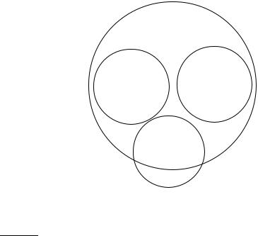
Figure 14.5 The multimodal class “a” consists of two different clusters (small upper circles centered on X’s). Rocchio classification will misclassify “o” as “a” because it is closer to the centroid A of the “a” class than to the centroid B of the “b” class.
applied to J > 2 classes whereas Rocchio relevance feedback is designed to distinguish only two classes, relevant and nonrelevant.
In addition to respecting contiguity, the classes in Rocchio classification must be approximate spheres with similar radii. In Figure 14.3, the solid square just below the boundary between UK and Kenya is a better fit for the class UK since UK is more scattered than Kenya. But Rocchio assigns it to Kenya because it ignores details of the distribution of points in a class and only uses distance from the centroid for classification.
The assumption of sphericity also does not hold in Figure 14.5. We can-
Online edition (c) 2009 Cambridge UP

296 |
|
|
14 Vector space classification |
|
|
mode |
|
time complexity |
|
|
||||
|
training |
|
Θ(|D|Lave + |C||V|) |
|
|
testing |
|
Θ(La + |C|Ma) = Θ(|C|Ma) |
|
Table 14.2 Training and test times for Rocchio classification. Lave is the average number of tokens per document. La and Ma are the numbers of tokens and types, respectively, in the test document. Computing Euclidean distance between the class centroids and a document is Θ(|C|Ma).
not represent the “a” class well with a single prototype because it has two MULTIMODAL CLASS clusters. Rocchio often misclassifies this type of multimodal class. A text classification example for multimodality is a country like Burma, which changed its name to Myanmar in 1989. The two clusters before and after the name change need not be close to each other in space. We also encountered the
problem of multimodality in relevance feedback (Section 9.1.2, page 184). Two-class classification is another case where classes are rarely distributed
like spheres with similar radii. Most two-class classifiers distinguish between a class like China that occupies a small region of the space and its widely scattered complement. Assuming equal radii will result in a large number of false positives. Most two-class classification problems therefore require a modified decision rule of the form:
Assign d to class c iff |~µ(c) −~v(d)| < |~µ(c) −~v(d)| − b
|
for a positive constant b. As in Rocchio relevance feedback, the centroid of |
||||||
|
the negative documents is often not used at all, so that the decision criterion |
||||||
|
simplifies to ~µ(c) |
− |
~v(d) |
| |
< b′ for a positive constant b′. |
|
|
|
| |
|
|
2 |
Adding all |
||
|
Table 14.2 gives the time complexity of Rocchio classification. |
|
|||||
|
documents to their respective (unnormalized) centroid is Θ(|D|Lave) (as op- |
||||||
|
posed to Θ(|D||V|)) since we need only consider non-zero entries. Dividing |
||||||
|
each vector sum by the size of its class to compute the centroid is Θ(|V|). |
||||||
|
Overall, training time is linear in the size of the collection (cf. Exercise 13.1). |
||||||
|
Thus, Rocchio classification and Naive Bayes have the same linear training |
||||||
|
time complexity. |
|
|
|
|
|
|
|
In the next section, we will introduce another vector space classification |
||||||
|
method, kNN, that deals better with classes that have non-spherical, discon- |
||||||
|
nected or other irregular shapes. |
|
|
||||
? |
Exercise 14.2 |
|
|
|
|
|
[ ] |
Show that Rocchio classification can assign a label to a document that is different from |
|||||||
its training set label. |
|
|
|
|
|
|
|
2. We write Θ(|D|Lave) for Θ(T) and assume that the length of test documents is bounded as we did on page 262.
Online edition (c) 2009 Cambridge UP