Kluwer - Handbook of Biomedical Image Analysis Vol

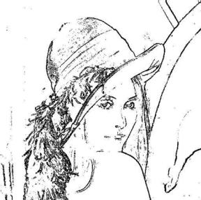
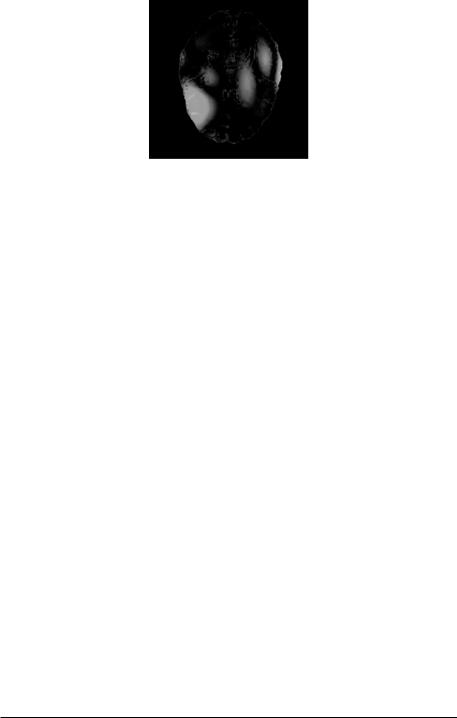
Figure 9.11: Example of a mask selecting 10 % of the pixels with the highest gradient values for the Lena image.

number of pixels, and to consider only those pixels in subsequent calculations. The contributions of individual pixels to the change of the criterion is directly proportional to the amplitude of the directional derivatives at the respective points, see (9.12). Therefore, a reasonable strategy is to construct the mask by thresholding the gradient of the image at each multiresolution level (see Fig. 9.11).

9.4.9 Invertibility and Regularization

In some applications, it is useful to add an extra regularization term Er to the difference measure E, and to look for a minimum of the combined criterion

The factor Er is used to make the solution well-posed, or to privilege likely solutions based on our a priori knowledge.

First, we consider a penalty term designed to enforce the invertibility of the deformation, generalizing the concept from [95] and similar to [113]. Its moti-

vation comes from the fact that if the Jacobian det( g) is positive everywhere,

x

then the deformation g is locally invertible. Evaluating this constraint at pixel coordinates and converting the strict constraints into soft ones using a barrier function yields the following penalty term

Experience shows that, for typical data, this term is never important at the solution point (to which the optimization converges). It mostly becomes useful at the beginning of the optimization process when the trial points vary a lot, especially with some optimizers. In such cases, the penalty term forces the algorithm to stay in the region of invertible deformations.

Depending on the particular task and the expected properties of the solution, various regularization terms can be used. We investigated, for example,

a stabilizer penalizing non-linear deformations

and a very simple norm measuring the distance of g from identity through the coefficients c

Ed = !cj!2 (9.24)

j

When the corresponding weight γ is small, the regularization mainly smoothes the deformation function in places where little information is present in the images. As it gets bigger, the regularization gradually overrides the data term and the deformation tends towards a smooth function in the sense of the particular regularization. An alternative to regularization is the virtual spring mechanism described in section 9.4.7.

9.4.10 Experiments

We now illustrate the application of the presented algorithm to various problems involving medical images of several modalities. We refer the interested reader to [88,95,96], where we study in detail the accuracy, speed and robustness of the algorithm by means of a comprehensive series of experiments in a controlled environment.

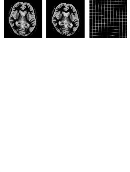
Figure 9.12: The original slice of anatomical MRI brain image ((top left), original superimposed over the true deformation (top right), the recovered deformation versus the true deformation (bottom left), and the mask used to calculate the warping index (bottom right). (Color Slide)

9.4.10.1 Registration of Artificially Deformed MRI Brain Slices

To illustrate the behavior of the algorithm, we show its performance when recovering a known deformation of a 2D slice of an anatomical spin-echo MRI volume of the brain.9 We use here artificially-deformed images because the knowledge of the ground truth permits us to better judge the performance of the algorithm.

The original image of size 256 × 256 pixels is shown in Fig. 9.12, top-left. We use a cubic spline control grid with one knot for every 32 pixels. We warp the image with a deformation belonging to the warp space and consisting of displacements up to 15 pixels.10 The warped image is superimposed on the original in Fig. 9.12, top-right. Then the automatic registration algorithm is run with the stopping threshold set to 0.5 pixels for all levels except the last, where we set it to 0.1 pixels. The recovered deformation was used to warp again the original image. Its warped version is shown superimposed on the image warped

9 First author’s brain. Images courtesy of Arto Nirkko from Inselspital Hospital, Bern,

Switzerland.

10 Approximately 14 mm.

Figure 9.14: The geometrical error after registration (green) with superposed contours of the original MRI image (red). The maximum (green) intensity corresponds to an error of 1.5 pixels. (Color slide.)

optimized (E) and of the warping index ( ), the quantity measuring the quality of the registration. The abrupt changes in the curves are caused by the transitions between levels of the multiresolution progression; they are small thanks to the

set stopping threshold, which in turn influences the optimization time. The threshold value is a subjective compromise between the accuracy and computation time. It is perfectly possible to stop optimizing only after 7 s and

skip the finest resolution level altogether, if the precision of = 0.7 pix-

els is acceptable. On the other hand, after about 4 more minutes of iteration, the error descends to less than 10−4 pixels. However, in the authors’

opinion, such super subpixel accuracy is almost never achievable on real images, because of the noise and the unknown characteristics of the acquisition process.

9.4.10.2 Registration of True Medical Data

Finally, we give a representative list of medical imaging registration tasks where the described algorithm was successfully used:

Registration of ECD11 and Xenon inhalation SPECT images [114] in the view of atlas creation [115].

11 ECD (Technetium Ethylene Cysteine Diethylester) is a radioactively marked intra-

venously injected agent.

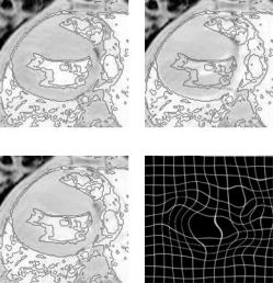
Figure 9.15: The superposition of the slices of anatomical MRI images before the registration (a), after the registration (b), and the resulting deformation field

(c). Quadratic splines were used with knot spacing of h = 64. (Color slide.)

Intersubject registration of anatomical (spin-echo) MRI images,12 Fig. 9.15.

Registration of MRI images from a heart beat sequence,13 see Fig. 9.16. The extracted deformation field can be used to extract trajectories of various points in the heart and to further determine the velocity and derived parameters, such as the accumulated displacement and strain, which is important for diagnostic purposes.

Registration of standard 2D ultrasound sequences of the heart [116].

Motion compensation for a sequence of myocardial perfusion MRI images14 [117, 118], enabling the time profiles of the intensities at each tissue point to be reliable calculated (Fig. 9.17). Virtual springs were used in this case.

Registration of two 3D computer tomography (CT) head volumes,15 see Figs. 9.18 and 9.19. We worked on a reduced volume data (128 × 128 × 45

instead of the original 512 × 512 × 45) with control knots placed every

8 × 8 × 8 voxels and the process took about 10 minutes to complete.16

12Images courtesy of Arto Nirkko, Inselspital Hospital, Bern, Switzerland.

13LECB, NIH, http://www-lecb.ncifcrf.gov/flicker/

14Courtesy of J.-P. Vallee,´ Unite´ d’imagerie numerique,´ University Hospital, Geneva,

Switzerland.

15 Images courtesy of Philippe Thvenaz, EPFL, Lausanne, Switzerland. The images were acquired using the same machine and the same protocol, but not preregistered.

16 On a 700 MHz Pentium based computer. Registering directly the undecimated volumes on the same computer takes about three hours with very minor increase in quality as relatively smooth deformations are sought. We are currently working on a optimized reimplementation of the algorithm that should reduce these times considerably.

Figure 9.16: The reference MRI image from a heart sequence with superimposed contours (a). The same contours over another image (the test image) from the same sequence before the registration (b) and after (c). The deformation field (d). Quadratic splines were used with knot spacing of h = 64, image size was 256 × 256 pixels. (Color slide.)

9.4.11 Summary of Elastic Registration

The algorithm that has been described is a state-of-the-art example of what is available in the field of fully automatic elastic pixel-based registration. It contains many features that have been proposed in the literature and it has been streamlined for an efficient execution.

Elastic registration has numerous applications in the biomedical imaging field, all based on the basic notion of aligning two images with one other, be it intersubject, intrasubject, or intermodality. It can be used for motion and deformation detection. The deformation field itself can be used for deformation and motion compensation as well as for quantitative measurements.

The criterion, the deformation model, the regularization (penalty), and the optimization algorithm should be all adapted to the task at hand for optimum results.

By producing a specialized program taking advantage of a specific configuration, the runtime can be probably decreased by an additional factor of 10.

Figure 9.17: The first line presents original images number 6,9,11, and 14 from a sequence of originally 60 images of myocardical perfusion MRI. The second line presents the difference images between the original images and their immediate predecessors; movement artifacts can be clearly seen. On the third line you can see the difference images from the motion corrected sequence using our algorithm; the movement artifacts are significantly reduced. The same effect is also visible comparing the differences of the sequence images with the first image of the sequence on the original (fourth line) and corrected (fifth line) sequences.

This, together with the constant advances in computer technology will enable truly interactive operation of automatic and semi-automatic elastic image registration with numerous applications in medicine, biology, and any other field where deformed images need to be compared.