

Kluwer - Handbook of Biomedical Image Analysis Vol
.3.pdf340 |
Kybic and Unser |
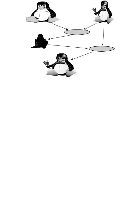
Figure 9.1: Two versions of a penguin Tux, the Linux mascot (above). Even though they are different, corresponding points can be identified (below). (Color slide.)
While image registration takes the test and reference images and yields a cor-
respondence (deformation) function, the image warping takes the test image
anda correspondence function and outputs a warped image fw (x) = f g(x)
which is a deformed version of the test image. The warped test image is aligned
Figure 9.2: Corresponding magnetic resonance brain slices from EPI (left) and anatomical (right) modalities. Landmarks (white crosses) have been manually placed at corresponding locations.
Elastic Registration for Biomedical Applications |
341 |
reference image |
test image |
registration
deformation
warping
warped image
Figure 9.3: Given an image and a deformation function, a deformed image is created by warping. Inversely, given two images, the corresponding deformation function is found by image registration. The registration attempts to make the warped image as similar as possible to the reference image. (Color slide.)
with the reference image and conversely, registering an original image with its warped version recovers the deformation used.
We will call a registration elastic, if the family of correspondence functions g is sufficiently general, capable of expressing (almost arbitrary) nonlinear relations4 as opposed to considering for example only linear functions g.
9.1.1 Applications of Image Registration
Historically, some of the first applications of image registration occurred in the domain of motion analysis [2]. The task there is to find changes between two subsequent frames in a video sequence, assuming that these changes can be completely explained by movements of the objects in the scene or of the observer. In most cases, the inter-frame changes are relatively small and the movement smooth. The extracted motion field can be used to measure the trajectories,
4 Note that elasticity is used here in a wider sense than just the mechanical linear elastic-
ity [1].
342 |
Kybic and Unser |
distances, speeds, and accelerations, etc. In video compression, this information enables us to take advantage of the temporal redundancy in the video sequence; it can be used for object tracking [3], image stabilization, or camera (observer) movement identification leading to 3D reconstruction of the scene. segmentation algorithms divide the image into regions according to their speed.
Registering a pair of stereo images also permits the 3D reconstruction of the scene. The spatial configuration of the cameras is known here; on the other hand, we have to deal with occlusions. The general case of n cameras presents additional challenges in maintaining the consistency.
9.1.1.1 Biomedical Applications
In the biomedical domain, there is a frequent need to compare images for analysis and diagnostic purposes. For an efficient comparison, the images need to be aligned. This can be accomplished by registration and subsequent warping.
Intrasubject analysis compares images of the same subject taken at different times in order to detect or quantify changes caused by the evolution of the disease or the effect of the therapy.
Intersubject analysis considers corresponding images from different subjects. Aligning and combining images from many subjects leads to atlases, which are annotated reference images. The individual subject images are then registered with the atlas for identification, segmentation, to detect abnormalities, and to quantitatively characterize the shape and size of their features.
Images of the same subject with different imaging modalities can be combined using intermodality registration to get a more complete picture of the subject’s anatomy and physiology.
Furthermore, registration helps to compensate for geometrical distortions [4] inherent to some imaging methods, as well as for unwanted motion during the acquisition.
9.2 Review of Registration Techniques
Most existing registration algorithms can be cast into the following general framework:
Elastic Registration for Biomedical Applications |
343 |
In the first step, some intermediate data is extracted from the two images being registered. This data lives in a feature space.
The algorithm’s representation of the correspondence between the two images is taken from a search space. This is the space in which the algorithm looks for a solution. An element from this space is returned at the end.
To find the solution in the search space, the algorithm needs a way to measure the quality of the correspondence for different points in this space. This measure is provided by a cost function.
Finally, the search strategy governs the movements of the algorithm in the search space in its quest for the optimum.
We classify existing registration algorithms according to their choice of the above four attributes, similarly as in [5]. We shall concentrate mostly on their biomedical applications. Figures 9.4 and 9.5 show the simplified classification according to the first two attributes in a tree form.
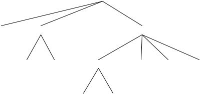
9.2.1 Feature Space
According to the feature space employed, we can identify three classes of registration algorithms: pixel-based, transform-based, and feature-based.
Feature space
pixels |
transforms |
features |
Fourier |
wavelet |
landmarks |
curves |
surfaces |
templates |
intrinsic extrinsic
Figure 9.4: Simplified classification of registration algorithms according to the
feature spaces used.
344 |
|
|
|
|
|
|
Kybic and Unser |
||
|
|
|
|
Warp space |
|
|
|
|
|
|
local |
|
semi-local |
|
|
global |
image dependent |
||
PDE |
variational |
quadtree |
B-splines |
wavelets |
|
|
|
|
|
|
|
|
|
|
|||||
linear |
polynomial |
harmonic |
RBF |
||||||
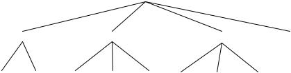
Figure 9.5: Simplified classification of registration algorithms according to the warp space used.
9.2.1.1 Pixel-Based Registration
Pixel-based algorithms work directly with the (totality of) pixel values of the images being registered. Preprocessing is often used to suppress the adverse effects of noise and differences in acquisition [6], or to increase or uniformize pixel resolution [7]. In the continuous framework, images are often considered as functions of the continuous image coordinates, providing a consistent approach to the discretization issues. The correspondence between the discrete and continuous versions of the image is established using interpolation. The crudest method is the nearest-neighbor interpolation, the most often used is the linear (resp. bior trilinear) interpolation. Among the high-end methods,
B-spline interpolation [8–10] provides the best trade-off between accuracy and the computational cost [11, 12].
The image model may also live in a higher-dimensional space than the original data, such as when representing 2D image as a surface in a 3D space [13], or using level sets [14].
9.2.1.2 Transform-Based Registration
Transform-based algorithms exploit properties of the Fourier, wavelet, Hadamard, and other transforms, making use of the fact that certain deformations manifest themselves more clearly in the transform domain. These methods are used mainly in connection with linear deformation fields. Nevertheless, there are examples of methods that estimate locally linear optical flow using Gabor filters [15,16], B-splines [17] and wavelets [18]. The transforms are usually linear and independent of the actual image contents.
Elastic Registration for Biomedical Applications |
345 |
9.2.1.3 Feature-Based Registration
Feature-based algorithms first reduce the dimensionality of the problem by extracting a small set of characteristic features from the images. The extraction mostly involves thresholding.
Landmark-based methods [1, 19–21] use a relatively small and sparse set of landmarks—important points manually or automatically identified in the images. Extrinsic markers are artificial features attached to the object, easily and precisely localizable. Unfortunately, they are often long to install and uncomfortable for the patient. If they are not available, we have to content ourselves with features intrinsic to the images. In that case, however, the automatic landmark identification is far less robust. The manual landmark identification is often tedious, time-consuming, imprecise, and unreproducible.
If the images cannot be characterized using points, it might be more appropriate to use curves such as edges [22], or volume boundaries [23]. Likewise, in the case of 3D data, surfaces can be used instead of working with the complete volumes. Popular features are also templates, small subimages of important regions [24, 25].
9.2.2 Search Space
An important attribute of a registration algorithm is the search space. It is also called a warp space because it contains warping or correspondence functions, the candidate solutions of the registration problem. A warping function from the search space is described by a (finite) set of real parameters (from a set of permissible values) by means of a warping model. We classify them according to the number of parameters and the spatial extent of the area influenced by a single parameter.
9.2.2.1 Local Models
At one end of the scale, we have non-parametric, local methods. The deformation function sought is basically unconstrained, or belongs to a very large and unrestrictive functional space, such as the Sobolev space W22 of twice differentiable functions. We seek the values of this deformation at a very fine grid, usually coinciding with pixel locations. These methods are formulated either
346 |
Kybic and Unser |
as variational, defining a scalar criterion to minimize, or using partial differential equations (PDE). The continuously defined deformation function minimizes a given criterion, or solves a given PDE. The essence of these methods is thus entirely in the criterion (resp., PDE). The PDE come from the optical flow approach (gradient methods) [26], viscous fluid model [27–29], elastic deformations with physical analogs [7, 30] or without them [31], or from the variational criterion [32]
The deformation function can be also modeled indirectly, e.g., as a potential field [33]. This reduces the dimensionality of the problem, at the expense of reducing the generality of the deformation. Displacement might be quantized
(limited) to integer number of pixels [34].
9.2.2.2 Global Models
At the other end, we have parametric, global methods that describe the correspondence function using a global model with a relatively small number of parameters [35]. The model mostly consists of expressing the warping function in a global linear [36], polynomial [37] or harmonic basis [38, 39]. For these methods, the deformation model corresponding to a specific warp space is as important as the criterion being minimized.
9.2.2.3 Semi-Local Model
In between the two extremes are semi-local models, using a moderate number of parameters with local influence. A grid of control points is usually placed over the image and a basis function associated with each of them. Their spacing corresponds loosely to knot or landmark density. By changing the spacing, we can approach either local or global models or choose the best trade-off.
Semi-local models are instrumental for the B-spline based approach described in section 9.4 and were also used, for example, for motion estimation [40].
9.2.2.4 Image Dependent Models
It is sometimes useful to adapt the warping model to the images considered. Hierarchically structured semi-local models, based on splines, wavelets, or
Elastic Registration for Biomedical Applications |
347 |
quadtrees [41] can be refined only where needed. In feature based methods, the basis functions of the warping model can be placed where the features are and the deformation field interpolated in regions where no information is available. Typical examples are radial basis functions such as thin plate splines [1,19,42], to be discussed more in section 9.3.
9.2.3 Cost Function
The quality of a registration result is assessed by a cost function. It is mainly composed of a data term, measuring the similarity of the images after warping. Sometimes a regularity term is added to privilege likely (smooth) deformations.
9.2.3.1 Data Term
For methods based on geometric features, we can use a (mean) distance between corresponding features in the source and target images. Note that landmark interpolation (section 9.3) is a limit case with infinite weights given to this distance, constraining it effectively to zero. If the pairing between the source and target features is unknown, the iterative closest point algorithm [43], can be used to determine it.
For pixel-based methods, the data term is a similarity measure on the two images. The simplest and fastest criterion is the appropriate (e.g., l1 or l2) norm of the pixel-wise difference, such as in the SSD (sum of squared differences) criterion. However, it assumes an equivalency of intensities in both images. If the intensities only correspond up to a possibly varying linear relationship perhaps, then it is appropriate to use correlation, respectively, local normalized correlation [7, 44]. More general and perhaps non-functional relation between the intensities warrants the use of the mutual information criterion [45–48]. This is encountered, for example, in intermodality registration [49].
All three criteria lead to statistically optimal estimates of the registration under corresponding image and noise models. Their complexity, computational cost, and fragility increases in the order in which they were presented. For local criteria, such as local normalized correlation, or local mutual information, the neighborhood size must be properly chosen. Image interpolation is used to calculate the warped image, see also section 9.2.1.1.
348 |
Kybic and Unser |
In template-based methods, the template can be compared with a specific region in the target image using any of the similarity measures suitable for pixel-based methods. For transform-based methods, a (semi-)norm in the transformed domain such as L2 (least-squares measure) is usually used.
9.2.3.2 Regularization
In most applications, it appears to be necessary to add an additional regularization term to the criterion, mainly to make the problem well-posed and to stabilize the algorithm. Regularization is also used to express our a priori knowledge. For continuous, local deformation models, regularization defines the warping space in the variational sense. For instance, in the case of landmark interpolation, minimization of the norm of the Laplacian ! g! is often used in practice [1, 19], leading to a thin-plate spline solution [50]. Minimizing other similar measures leads to generalized splines [51] determined either directly or using PDEs. See also section 9.3.
Other regularizers are constructed by applying a non-linear (often quadratic and sometimes image dependent) function on the derivative operator. This is done mainly to preserve discontinuities [52]. Regularizers based on thresholding in wavelet domain are also used. Implicit regularization for iterative methods works by alternatively driving the intermediate solution towards the data, and applying a smoothing operator.
9.2.4 Search Strategy
Given a cost function, there are several basic ways of minimizing it.
9.2.4.1 Direct Solution
In some cases, notably if the cost function is quadratic or if higher order terms in the Taylor expansion of the criterion can be neglected, then the solution can be found in one step [38, 53]. Transform methods using directional filters are often engineered in this way [54, 55].
9.2.4.2 Exhaustive Search
If the search space is finite, exhaustive search can be used. For example, when small templates are extracted from the reference image, their positions in the
Elastic Registration for Biomedical Applications |
349 |
target image can be found by trying all possible shifts in some small neighborhoods [34, 56].
9.2.4.3 Dynamic Programming
For integer 1D problems, dynamic programming is applicable [57] with complexity proportional to the number of decisions to be taken (size of the image) and the number of possible outcomes (shifts). The stereo matching problem with cameras with known relative geometry also falls into this category [58]. These are nice examples of how the a priori knowledge about the image formation process simplifies the registration problem by imposing very strong geometrical constraints on the correspondence field.
9.2.4.4 Partial Differential Equations
A partial differential equation can describe an evolution in time of the deformation field converging to the desired solution [32, 52]. (Time-independent PDE’s derived directly by Euler-Lagrange formulas from the variational formulation are seldom used.) The PDE parameters can vary with time, to enforce robustness at first and relax the constraints toward the end, to allow for precise registration. Various numerical methods can be used to solve the PDEs, the principal ones being finite difference relaxation method [59], finite elements method (FEM) [60, 61], hierarchical finite element bases [62], multigrid methods [63], and wavelets [64, 65].
9.2.4.5 Multidimensional Optimization Methods
Many non-linear registration methods lead to a non-linear multidimensional optimization problem. Various optimization methods are used, depending on the size and structure of the problem. The most popular choices include the Powell method, gradient descent, conjugated gradients, and variations of the Newton method, such as the Marquardt-Levenberg algorithm [59, 66].
Some minimization algorithms are described using different paradigms, such as ‘demons’ [67], but usually can be explained in terms of a coordinate descent.
9.2.4.6 Multiresolution
Multiresolution [7,36,68] on the feature space (usually image size) helps to speed up the process and to increase its robustness. It is based on approaching the