

Kluwer - Handbook of Biomedical Image Analysis Vol
.3.pdfImage Segmentation |
259 |
are below the required tolerance, the triangle is not subdivided. Otherwise, the voxel that is farthest from the triangle is connected to the three vertices of the triangle to obtain three smaller triangles. This is depicted in Fig. 7.4d. The reason for subdividing the edge contours first is to avoid very long and narrow triangles in the final subdivision.
By subdividing a triangle, finer triangles are obtained. The process is repeated until distances of all shape voxels to the associating triangles become smaller than the required tolerance. Note that this subdivision is performed in parallel in the sphere as well. Therefore, whenever a triangle in the shape approximation is subdivided, the corresponding triangle in the sphere approximation is also subdivided. For that reason, there always exists a one-to-one correspondence between triangles in the shape approximation and triangles in the sphere approximation. By knowing the parameters of mesh vertices in the sphere, we will know the parameters of corresponding mesh vertices in the shape. This process assigns spherical parameters to the mesh vertices approximating the shape. The process is graphically shown in Fig. 7.5. The only requirement of the described parametrization is for the given shape to have spherical topology.
By knowing the parameters at vertices of a triangle, parameters at points inside the triangle can be computed from barycentric coordinates [16] of parameters at the vertices. Parameters of voxels in a triangular patch are obtained by projecting the voxels to the associating triangle and assigning parameters of the triangle points to the voxels. If a triangular patch does not fold over,
(a) |
(b) |
(c) |
(d) |
(e) |
(f ) |
(g) |
(h) |
(i) |
(j) |
Figure 7.5: (a) A sphere. (b–e) Subdivision of the sphere. (f) A digital shape. (g–j) Subdivision of the shape. The shape and the sphere are subdivided in parallel.
260 |
Jackowski and Goshtasby |
this mapping will be unique. If fold overs occur, the subdivision process should be continued until all fold overs disappear. When the maximum distance between a triangle and the associating patch is less than two voxels, fold overs cannot occur. More details about this parametrization algorithm and its characteristics can be found in [17].
The parameters obtained by this algorithm uniquely map shape points to triangular faces. The mapping is continuous but not smooth. To obtain a smooth parametrization, the parameters obtained here should be used as initial values to the nonlinear optimization described by Brechbuhler¨ et al. [3]. The surface-fitting method used in this work, however, does not require a smooth parametrization of the points. It only requires that the parameters vary continuously.
If the vertices of a triangular mesh approximating a digital shape are used as the control points of a RaG surface and the parameters at mesh vertices are used as the nodes of the surface, a smooth parametric surface can be obtained that approximates the shape. The surface obtained in this manner only approximates the mesh vertices. We can improve this shape recovery process by making the surface interpolate the mesh vertices. In the following section, a least-squares method that determines the control points of a RaG surface interpolating the mesh vertices is described.
7.2.3 Least-Squares Computation of the Control Points
Suppose a digital shape is available and the shape voxels are parametrized according to the procedure outlined in the preceding section. Also, suppose the shape is composed of N voxels: {P j : j = 1, . . . , N} with parameter coordinates {(uj , v j ) : j = 1, . . . , N}. We would like to determine a RaG surface with control points {Vi : i = 1, . . . , n} that can approximate the shape points optimally in the least-squares sense. Let’s suppose P j = (X j , Yj , Z j ), P(u, v) =
[x(u, v), y(u, v), z(u, v)], and Vi = (xi, yi, zi). Then the sum of squared distances between the voxels and the approximating surface can be written as
N
E2 = {[x(uj , v j ) − X j ]2 + [y(uj , v j ) − Yj ]2 + [z(uj , v j ) − Z j ]2} |
(7.5) |
|||
j=1 |
|
|
|
|
|
|
|
||
N |
N |
N |
|
|
= $ j=1 |
[x(uj , v j ) − X j ]2 + j=1 |
[y(uj , v j ) − Yj ]2 + j=1 |
[z(uj , v j ) − Z j ]2 |
(7.6) |
= Ex2 + Ey2 + Ez2. |
|
|
(7.7) |
|
Image Segmentation |
261 |
Since the three components of the surface are independently defined, to minimize E2, we minimize Ex2, Ey2, and Ez2, separately. To minimize
N
Ex2 = |
[x(uj , v j ) − X j ]2, |
|
(7.8) |
|
|
j=1 |
|
|
|
since |
|
|
|
|
|
|
|
|
|
x(uj , v j ) = |
n |
|
|
|
xigi(uj , v j ), |
|
(7.9) |
||
|
|
i=1 |
|
|
we minimize |
|
|
|
|
|
|
|
|
|
N |
n |
|
2 |
|
Ex2 = j=1 |
" i=1 |
xigi(uj , v j ) − X j # |
. |
(7.10) |
This involves determining the partial derivatives of Ex2 with respect to the xi’s, setting the partial derivatives to zero and solving the obtained system of equa-
tions. This results in |
|
|
|
|
|
N |
n |
|
gk(uj , v j ) |
[xigi(uj , v j ) − X j ] = 0; k = 1, . . . , n. |
(7.11) |
j=1 |
i=1 |
|
This represents a system of n linear equations, which can be solved for {xi : i = 1, . . . , n}. Since RaG basis functions monotonically decrease from a center point, if σ is not very large, Eq. (7.11) will have a diagonally dominant matrix of coefficients, ensuring a solution. In the same manner, {yi : i = 1, . . . , n} and
{zi : i = 1, . . . , n} can be determined by minimizing Ey2 and Ez2, respectively. Note that the above process positions the n control points of a RaG surface so that the surface will approximate the N image voxels with the least sum of squared errors. n depends on the size and complexity of the shape being approximated. n is typically a few hundred.
Since shape voxels are mapped to a sphere, spherical parameters are obtained for them. Assuming the approximating surface is represented by P(u, v), the distance of voxel Vi = (xi, yi, zi) to the surface is estimated from E(ui, vi) = ||Vi − P(ui, vi)||. The adjacency information between the control points is provided in the u and v parameter coordinates. Therefore, index i is arbitrary and the control points with their associated nodes can be rearranged in Eq. (7.1) without having any effect in the obtained surface.
When the standard deviation in a RaG surface is very small, the surface follows individual voxels. The selected standard deviation should be large enough
262 |
Jackowski and Goshtasby |
to smooth digital and image noise in segmentation. As the standard deviation of Gaussians is increased, a smoother surface will be obtained approximating the same set of voxels. Usually, the standard deviation of Gaussians in a RaG surface should be made proportional to the average distance between adjacent nodes. The denser the control points, the smaller the distance between their nodes, and thus, a smaller standard deviation should be used. Experimental results show that standard deviations from the average distance between adjacent nodes to five times that are appropriate for surface fitting. We will select this parameter interactively during shape editing.
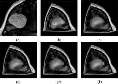
Figure 7.6a shows a region representing the bounding surface of a brain tumor. Subdivision of this region to a triangular mesh with a tolerance of 3 voxels is shown in Fig. 7.6b. The tolerance shows the maximum distance between the given digital shape and the approximating triangular mesh. Approximation of the tumor with a RaG surface of standard deviation 0.002 is shown in Fig. 7.6c. Increasing the standard deviation to 0.0025, 0.003, and 0.004, we obtain the
Figure 7.6: (a) A segmented brain tumor in an MR image. (b) Approximation of the tumor by a triangular mesh with a tolerance of 3 voxels. (c)–(f) RaG surfaces approximating the tumor with standard deviations 0.002, 0.0025, 0.003, and 0.004, resulting in RMSE of 1.9725, 1.9711, 2.1439, and 2.2497 pixels, respectively.
Image Segmentation |
263 |
results shown in Figs. 7.6d, 7.6e, and 7.6f, respectively. Root-mean-squared-error (RMSE) for Figs. 7.6c–7.6f are 1.9725, 1.9711, 2.1439, and 2.2497 voxels, respectively. The RMSE obtained in a RaG approximation of a digital region is usually much smaller than the tolerance used to approximate a digital shape by a triangular mesh. Figures 7.6c–7.6f appear very similar, but from the RMSE obtained, we see that their local geometries are somewhat different. The shape in Fig. 7.6f is much smoother and rounder than the shape in Fig. 7.6c.
At the standard deviation that matches the level of detail in a shape, the smallest surface-fitting error is obtained. This minimum error can be determined by a steepest-descent algorithm. However, since the given region is known to contain errors, finding the surface that is very close to the region may not be of particular interest. Currently, after the control points of an approximating surface are determined, the user interactively varies the smoothness (standard deviation) of the surface and views the obtained surface as well as the associating RMSE. In this manner, the standard deviation of Gaussians can be interactively selected to reproduce a desired level of details in a constructed shape.
7.2.4 Shape Editing
Once the result of an automatic segmentation is represented by a free-form parametric surface, the surface can be revised to a desired geometry by appropriately moving its control points. In the system we have developed, an obtained surface is overlaid with the original volumetric image. Then, by going through different image slices along one of the three orthogonal directions, the user visually observes the intersection of the surface with the image slices and verifies the correctness of the segmentation. When an error is observed, one or more of the control points are appropriately moved to correct the error. As the control points are moved, the user will observe changes in the surface immediately.
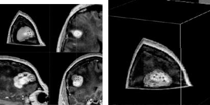
An example of shape editing by the proposed method is shown in Fig. 7.7. Figure 7.7a shows the surface approximating a brain tumor within the original volumetric image. The user selects a number of control points using a small sphere that is attached to the cursor and whose center lies in the image slice being reviewed. By placing the cursor near the area where an error has occurred in one of the slices and pressing the mouse button, the sphere is activated and the control points falling in the sphere are selected. By changing the radius of sphere, the number of control points selected for movement are changed. Control points
264 |
Jackowski and Goshtasby |
(a) |
(b) |
Figure 7.7: (a) Overlaying of the approximated tumor surface and the volumetric image. The blue dots show the selected control points during surface editing. The upper-left window shows the 3D view of the image volume with all three orthogonal slices. The other three windows show the individual orthogonal views in axial, sagittal, and coronal directions. (b) Another 3D viewing mode showing the surface in wireframe form to enable viewing of image information inside and behind the surface. The red dots show the control points of the surface.
selected by the sphere are then moved with the motion of the mouse. Control points inside the sphere are not all moved by the same amount and in the same direction. A point is moved in the appropriate direction by connecting the point to the center of the sphere and by using the amount proportional to the cosine of the angle between that direction and the direction of the motion of the mouse. Only those control points falling inside the hemisphere with positive cosines are moved. This avoids motion of control points with negative cosines in the opposing direction. It also ensures that discontinuities will not occur between points that are moved and points that are not. Intermediate results in surface modification are shown in Fig. 7.7a. Surface revision can be performed gradually and repeatedly while observing the image information. The sensitivity of the surface to the motion of the mouse can be changed by increasing or decreasing the weights assigned to the control points. To better view the intersection of the surface with the image planes, the surface can be shown in wireframe form as depicted in Fig. 7.7b. The edited surface can be digitized as shown in Fig. 7.8b to create the final segmentation in digital form.
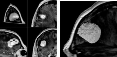
Image Segmentation |
265 |
(a) |
(b) |
Figure 7.8: (a) The tumor after necessary modifications. This is the final result in parametric form. (b) Digitization of the tumor. This is the final result in digital form.
7.3 Results
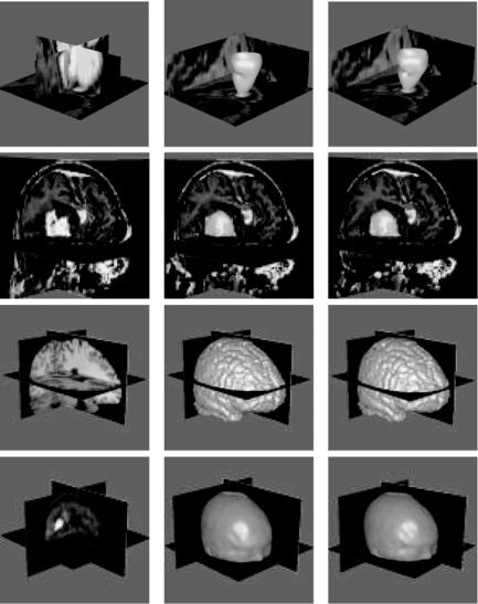
A few examples of image segmentation by the proposed method are shown in Fig. 7.9. The first column shows the original images, the second column shows the initial segmentation results, and the third column shows the results after the necessary revisions. The images represent a short-axis cardiac MR image (first row), an MR brain image containing a tumor (second row), an MR image containing only the brain (third row), and a PET image of the head (fourth row). The ventricular blood pool and the brain tumor were initially obtained by a smoothing operation and an optimal intensity thresholding method. In the thresholding method, first a subvolume including the object of interest is selected. Then the intensity threshold value that produces the minimum change in the region of interest as a result of change in threshold value by 1 is determined. The optimal threshold value is considered to be the intensity where the most stable segmentation is obtained. At the optimal threshold value, a small change in threshold value will change the segmentation result minimally. This threshold value corresponds to the intensity at object boundaries where intensities change sharply. Therefore, a slight error in estimation of the threshold value will not change the segmentation result drastically.
The brain image was roughly segmented slice by slice by hand, and the PET image was segmented by our 3D implementation of the Canny edge detector
266 |
Jackowski and Goshtasby |
Figure 7.9: First row: A short-axis cardiac MR image and segmentation of the left ventricular cavity. Second row: An MR brain image and segmentation of the tumor. Third row: An MR brain image and segmentation of the brain. Fourth row: A PET image and extraction of the surface of the head. The first column shows the original images, the middle column shows the initial segmentation results, and the right column shows the results after the necessary modifications.
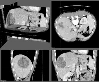
Image Segmentation |
267 |
Figure 7.10: An abdominal CT image.
[6]. The Canny edge detector produces a large number of edges. First, weak edges were removed by interactively varying the gradient threshold value and observing the obtained edges. Then, an edge surface of interest was selected by pointing to the surface with the mouse and extracting it from the image. In these figures, results of the initial segmentation are shown after RaG surface fitting by the least-squares method. RaG surfaces were then interactively revised as needed while viewing the overlaid surface and volumetric image. Final segmentation results are shown in the third column of Fig. 7.9.
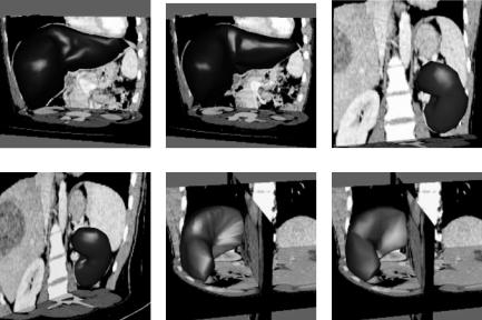
Another set of examples is shown in Figs. 7.10 and 7.11. Figure 7.10 is an abdominal CT image. Segmentation of different regions via intensity thresholding or edge detection, subdivision of obtained regions to triangular meshes, and fitting of RaG surfaces to the mesh vertices are shown in Fig. 7.11. Regions corresponding to the liver, one of the kidneys, and the spleen were selected one at a time and, after representing each by a RaG surface, were edited to remove inaccuracies in segmentation. Final segmentation results are shown in the column on the right in Fig. 7.11.
The time needed to obtain an initial segmentation and the time needed to modify the initial segmentation to obtain the final result vary from image to image. In the image shown in Figs. 7.9 and 7.11, approximation of the initial
268 |
Jackowski and Goshtasby |
Figure 7.11: First row: Polygon mesh and RaG surface approximation of the liver. Second row: Polygon mesh and RaG surface approximation of the kidney. Third row: Polygon mesh and RaG surface approximation of the spleen.
regions by triangular meshes took from 10 to 30 seconds and approximation of the regions with RaG surfaces by the least-squares method took from 40 to 60 seconds. Interactive revision of the initial surfaces to obtain the final surfaces took from 1 to 2 minutes. All these times are measured on an SGI Octane computer with R10000 processor and 128 MB RAM. Although the time to subdivide a region into a triangular mesh and the time to fit a RaG surface to a volumetric region are fixed for a given region, the time needed to revise an initial surface to a desired one depends on the speed of the user and the severity of errors in the initial segmentation.
The final result of a segmentation obtained by the proposed system is user dependent. In a typical image, the user judges what a correct segmentation is based on his/her past experiences while taking into consideration the information present in the image. Since users have different experiences in image interpretation, results obtained by different users will be different. Even the same user may segment an image differently at different times. The intrauser variability and interuser variability are not the characteristics of the proposed system, but rather those of the users. The proposed system provides tools with