Kluwer - Handbook of Biomedical Image Analysis Vol

Floating Image

Initial Transform Transform Update Transform

Figure 4.1: Flow-chart of image registration by mutual information maximization.

Our implementation is based on Java, using a lot of Java 2D graphics and image processing capabilities. Java 2D API includes a set of classes that can be used to create high quality graphics. It has features like geometric transformation, alpha composition, and image processing (see [33, 34]).

4.2.2 Transformation

In image registration different transformations can be considered: rigid-body transformation, affine, and nonlinear warping, with increasingly technical difficulty. In this chapter we consider affine transformation with a scaling factor, rotation angle, and two translational offsets. It is reported that the affine transform is sufficient for most retinal registration [23].

In homogeneous coordinate systems, an isotropic scaling transformation matrix is

where s is the scaling factor. The rotation matrix is

where θ is the rotation angle. The transformation matrix corresponding to the translation is

where tx and ty are translation offsets.

A successive transformation amounts to multiplication of corresponding matrices. We enforce the order of operations as scaling, rotation, and then translation, in matrix form, T · R · S. We seek (s, θ, tx, ty) parameters and these parameters are applied to the floating image in the order discussed above.

An affine transform can be easily composed in Java:

AffineTransform at = new AffineTransform ();

at.translate(tx, ty);

at.scale(scale, scale);

at.rotate(Math.PI/180.0*angle);

To create a transformed image, one can invoke the filter method of the AffineTransformOp, which can be constructed from the rendering hints and affine transform. The Java code is similar to

RenderingHints rh = new RenderingHints(/* specify here */); AffineTransform at = new AffineTransform();

// define transform here

AffineTransformOp atop = new AffineTransformOp(at, rh); BufferedImageOp biop = (BufferedImageOp) atop; BufferedImage bi = biop.filter(bi, null);

For retinal image registration, the maximum horizontal translation tx is 100 pixels, the vertical translation ty is in the order of 10 pixels, the maximum rotation angle θ is 5◦ and a typical scaling factor falls in [0.95, 1.05]. In the optimization process, we clamp the scaling factor to a certain range. A negative scaling factor is relatively impossible. A zero scaling is also impractical and Java 2D would generate a runtime exception.

4.2.3 Interpolation

After a transformation is applied, the grid point in the floating image will typically not coincide with another grid point in the transformed space. For a simple example, consider translation tx = 0.25. Grids (0, 0), (1, 0) become (0.25, 0), and (1.25, 0). Since the pixel values of the reference image are known on grid, and under certain transformations, only the pixel value of the transformed floating image on grid are of interest, the pixel values of the transformed floating image on grid have to be estimated. The technique is called interpolation, which is to estimate a pixel value based on the pixel values of its surrounding pixels.

There are different kinds of interpolation methods: nearest neighbor (0-order), bilinear (first-order), etc. Tsao evaluated the interpolation effects on registration performance [31]. Nearest neighbor uses the pixel value at the nearest grid pixel to approximate the pixel value at the new position. That is, the pixel value at (x, y) is approximated by that at ((int)(x + 0.5), (int)(y + 0.5)). The nearest neighbor interpolation is insensitive to the magnitude of translation up to one pixel. Therefore, it is not sufficient in order to achieve subpixel registration accuracy.

Bilinear interpolation assumes the pixel value in each x and y direction changes in a linear fashion. To get the pixel value at point (x, y), one can (a) interpolate the value at (x, j) from (i, j) and (i + 1, j), (b) interpolate the value at (x, j + 1) from (i, j + 1) and (i + 1, j + 1), and (c) interpolate the value at (x, y) from (x, j) and (x, j + 1), where integer i and j satisfy i ≤ x < i + 1 and j ≤ y < j + 1.

In Java 2D, the interpolation method is governed by the rendering hints. To specify a nearest neighbor interpolation, the rendering hints can be defined by

RenderingHints rh=new RenderingHints (

RenderingHints.KEY-INTERPOLATION,

RenderingHints.VALUE-INTERPOLATION-NEAREST-NEIGHBOR);

Similarly, to use a bilinear interpolation, the rendering hints can be specified as

RenderingHints rh=new RenderingHints (

RenderingHints.KEY-INTERPOLATION,

RenderingHints.VALUE-INTERPOLATION-BILINEAR);

Both interpolation methods were used. If a nearest neighbor interpolation is used, the optimization process tends to be quicker, but the success rate of registration tends to be lower. Thus, all results reported in this chapter are obtained using bilinear interpolation.

4.2.4 Estimation of Joint and Marginal Distributions

To calculate the mutual information, one has to have the marginal and joint pdfs. Since they are unknown, they have to be estimated from the data under study. We estimate these pdfs from their corresponding histograms.

To compute the histograms, the pixel pairs at the same grid are binned. Assume the bin size is Br ·B f , where Br and Bf are the bin size for the pixels in reference image and floating image, respectively.

A fixed bin size (32) is used. We will not discuss bin size effect since our preliminary results indicate that there are no apparent effects on the registration performance. For the byte image as the retinal GIF files normally are, there are 256 values in each color channel. However, when images are digitized and then translated from color to grayscale, there is some error. The image does not have very bright and very dark regions. Moreover, the lossy JPEG image compression is frequently used. These facts lead to a sparsely filled histogram if a 256 × 256 bin is used. Therefore, before we bin the pixel pairs their values are processed and then binned.

Assume the maximum pixel value is Imax and the minimum pixel value is Imin. Since we only have B bins, each bin needs to accommodate step =(Imax − Imin)/B different pixel values. Given a pixel value v, obviously it will be binned to bin (v − Imin)/step. Notice that we did not distinguish reference and floating images. The formula and schemes are applicable to both images. Also notice that interpolation never increases or decreases the max and min pixel values (except it may introduce zero-valued pixels due to transformation). This assertion is clear for the nearest neighbor interpolation. It is also true for the

bilinear interpolation since, based on the formula, the new pixel value is a convex combination of old ones. This property is used in the implementation and steps are only calculated once and never changed thereafter.

The overlapping pixels are scanned and the joint histogram is then computed.

Let the joint histogram be H(i, j). The marginal histograms are then

Hr (i) = H(i, j),

j

Hf ( j) = H(i, j).

i

Here the subscripts r and f stand for reference and floating, respectively. Let N be the total number of pixel pairs examined in the overlapping region then the joint and marginal pdfs are estimated as

H(i, j)

,

N

Hr (i)

,

N

Hf ( j)

.

N

Substituting those estimated joint and marginal pdfs into the definition of mutual information, its value can be readily computed. Since the iterative optimization routine is for minimization problem, the negated mutual information is actually computed.

4.2.5 Optimization

The sole goal of mutual information approach to image registration is to find a transformation under which the mutual information between the reference image and the transformed floating image is maximized. This is a typical optimization problem and many optimization methods have been employed, including exhaustive search, gradient descent, simplex downhill, Powell’s method, simulated annealing, and genetic algorithms [36]. This chapter studies the simplex downhill optimization since it is reported that it is faster than other algorithms with similar accuracy [36]. Simplex is also the easiest method to understand and does not require any derivative calculation.

The simplex downhill method may be trapped at local minimum. Simulated annealing method can avoid the problem, but it is computationally expensive. To avoid that we incorporate multiresolution strategies into the iterative process.

4.2.5.1 Exhaustive Search

The exhaustive search can be used to find the true global optimum solution. This brute-force search is very expensive. If we want 0.1 pixels, 0.1 rotations, and 0.001 scaling accuracy, we would have 1010 iterations.

4.2.5.2 Simplex

The downhill simplex method implements an entirely self-contained strategy and does not make use of any 1D optimization algorithm [31]. It requires only function evaluation, not derivatives.

A simplex is a geometrical figure, consisting of N + 1 vertices in N dimensions and all their interconnecting line segments, polygonal faces, etc. In the optimization process, a simplex reflexes, expands, and contracts, around a vertex, trying to enclose the optimum point within its interior.

The downhill simplex method must be started with N + 1 points, defining an initial simplex. For our image registration problem, there are four unknown registration parameters. Given an initial guess of the registration parameters vector (tx, ty, θ , s), a non-degenerate simplex can be formed by points (tx + 1, ty,

θ , s), (tx, ty + 1, θ , s), (tx, ty, θ + 1, s), and (tx, ty, θ, s + 0.1). In our implementation, the initial registration parameter vector is (0, 0, 0, 1), i.e., all translation offsets are 0, rotation angle 0, and the scaling factor 1.

Note that we use different guesses for the problem’s characteristic length scale in different directions since we don’t expect that the optimized scaling factor will be significantly deviated from 1. We use degrees rather than radians such that the characteristic length scale of rotation angle is comparable with those for translations (1 radian amounts to 57.3◦). In Java a zero scaling factor will generate an exception. In reality, a non-positive scaling factor does not make any sense. From the characteristic of the retinal image registration problem, one knows that the scaling factor falls in the range of 0.95–1.05. The simplex optimization routine cannot guarantee that. Thus, at each iteration the proper range of the scaling factor is checked. A relaxed lower and upper bounds is used. We clamp the scaling factor at a lower bound of 0.9 and an upper bound of 1.10.

The termination condition in any multidimensional optimization routine can be delicate. One can terminate the iterative process when the vector distance moved in a step is fractionally smaller in magnitude than some preset tolerance. Alternatively, one can require that the decrease in the function value in the

terminating step be fractionally smaller than a preset tolerance. In the simplex optimization, the relative difference between the highest and lowest vertices is compared against a tolerance (0.0001).

4.2.5.3 Multiresolution Strategies

The above optimization process can be attracted to a local minimum (thus local maximum of mutual information). To avoid that multiresolution or subsampling optimization scheme can be used. The idea of multiresolution strategy is simple: Find the optimal registration on coarse images first. Then using the found solution as the starting point, find the optimal registration for the fine images. The coarse images are derived from the original images, by averaging several pixels in the original images. As a variation of this multiresolution, subsampling is also used sometimes. Instead of taking the average, a single pixel is picked to form a coarse image. In the subsampling scheme, the images are never scaled down. The original images are subsampled periodically, with a gradually increasing sampling frequency. The optimization result at the lower sampling frequency is used as the starting point for the higher sampling. Since the images are subsampled, some information is lost.

We propose a multiresolution subsampling scheme. The idea is to combine the advantages of multiresolution and subsampling. Our experimental results indicate that this scheme can increase the convergence speed considerably. The pseudo code for this scheme follows:

For resolution r1 > r2 > ... > rn

Rescale the translation offsets (divided by the folding number)

Prepare the coarse images

For sampling s1 > s2 ... > sm

Do simplex optimization

Rescale translation offsets to correct different resolution effect

In the implementation, all these resolutions r and sampling frequencies s can be adjusted. In the experimental results reported below, the resolutions are 27, 9, 3, 1 and the sampling frequencies are 3 and 1.

The simplex optimization in the inner loop is identical to the one described earlier, except the images are scaled down by some folding factor which is equal

were taken using a Nidek stereo fundus camera. The original images were taken with color slide film and then digitized with a Polaroid slide digitizer. The images used for registration had 256-gray levels and comprise about 5% of the total surface of the retina centered on the optic nerve head.

Following is a brief description of the image files. All image files are labeled based on the patient identification, l/r, l/r, and a number. The first “l” or “r” indicates that those are the images of the patient’s left or right eye. The second “l” or “r” designates the left or right stereo images. These images were taken simultaneously onto a single photographic slide and were separated into two images manually after digitization. The last digits, 5, 6, or 7, indicate whether the images were taken in 1995, 1996, or 1997.

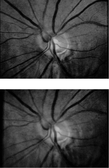
Image set 1 . There are four images in this patient file: ll5, ll7, lr5, and lr7. They are the same images as in Fig. 4.2 [5]. These images of left eyes were taken in 1995 and 1997, 18 months apart, during which time the patient had an operation to relieve pressure related to glaucoma. They are displayed in Fig. 4.2 here. This image set gives us two stereo image pairs (ll5/lr5, ll7/lr7) and two temporal pairs (ll5/ll7, lr5/lr7).

Image set 2 (B853). There are six images in this set: ll6, ll7, lr6, lr7, rl7 and rr7, which gives us three stereo pairs (ll6/lr6, ll7/lr7, and rl7/rr7) and two temporal pairs (ll6/ll7 and lr6/lr7).

Image set 3 (H3397). There are four images in this set: ll6, ll7, lr6, and lr7, which gives us two stereo pairs (ll6/lr6 and ll7/lr7) and two temporal pairs (ll6/ll7 and lr6/lr7).

Image set 4 (P374). There are eight images in this set: ll5, ll6, lr5, lr6, rl5, rl6, rr5, and rr6, which gives us four stereo pairs (ll5/lr5, ll6/lr6, rl5/rr5, and rl6/rr6) and four temporal pairs (ll5/ll6, lr5/lr6, rl5/rl6, and rr5/rr6).

All together we have 11 stereo image pairs and 10 temporal image pairs, which is a subset of the images used by Ritter et al. [5].

4.3.2 Mutual Information as a Measure

In this section we study mutual information as a measure for retinal image registration. Look at an extreme case first: an image registers to itself. At registration, the pixel values in two images have an exact one-to-one (identical) relation. In their joint histogram, there would be a straight, diagonal line. For any two

(a)

(b)

Figure 4.2: Typical temporal and stereo retinal images. (a) ll5, (b) lr5, (c) ll7, and (d) lr7 in image set 1.

images, we would not expect to see any structure in the joint histogram when they are not registered.

For two images of the same modality, one would expect a similar situation. However, due to noise, change of imaging condition, or change of the imaged