

Kluwer - Handbook of Biomedical Image Analysis Vol
.3.pdfThree-Dimensional Registration Methods |
127 |
similar gray values. In total, there are 4, 4, and 8 volumes for volunteer S1, S2, and S3, respectively. The permutation of the volumes gives many possible volume pairs for registration experiments.
3.3.4.3 Volumes for Registration Experiments
We registered 17 volume pairs under five different conditions as defined above. Five pairs are treatment-diagnosis; seven pairs are full bladder-empty bladder; two pairs are diagnosis 1 week-diagnosis; and three pairs are diagnosisdiagnosis. For each case, other conditions were controlled. For example, for the case of diagnosis 1 week-diagnosis, both volumes were acquired with empty bladder and comparable conditions. Rigid body and warping registration were applied to each of the volume pairs. Results were evaluated as described next.
3.3.4.4Effect of Control Point Selection on Registration Quality
In well over 100 registration experiments using different numbers and placement of CPs, we investigated effects on non-rigid registration quality. For each of the three volunteers, we selected one typical volume pair from the diagnostictreatment positions for systematic experiments. We progressively increased the number of CPs from 15 to 250. We found that less than 120 CPs did not produce good visual matching of our high-resolution MR images showing great anatomical detail. More than 220 CPs did not give significantly improved results but required more time for manual selection and optimization. When we used ≈180 CPs placed strategically using rules described later, we obtained excellent results over the entire pelvis and internal organs. As a result of our experience, we modified the registration method to be suitable for many CPs.
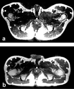
Some rules follow for strategic placement of CPs. For registration of treatment and diagnostic image volumes, most CPs were selected using transverse slices because they best showed the pelvic displacement when moving the legs to the treatment position (Fig. 3.9). About 25 CP pairs were placed near the edge and point features having recognizable correspondence on each of 5–8 transverse slices with a z interval of ≈8 mm, covering the entire pelvic region. Additionally, we placed about 25 CPs from sagittal slices
128 |
Fei, Suri, and Wilson |
Figure 3.9: Control point selection when images are acquired in the treatment and diagnostic positions. Image (a) is from the reference volume acquired in the treatment position with legs raised. Image (b) is to be warped and is from the volume acquired in the diagnostic position with the subject supine on the table. Transverse slices best show the deformations, especially at the legs. As described in the text, control points indicated by the white dots are selected around the pelvic surface and the prostate. Each control point is located at one voxel but displayed much bigger for better visualization. Volumes are from volunteer S2.
because they provided other structures that can be missed in the transverse images. It was also important to include CPs from organs other than the prostate because they constrained warps. We always placed CPs at critical regions such as the prostate center, pelvic surface, bladder border, and rectal walls.
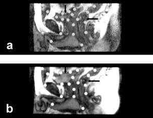
For registration of image volumes with full and empty bladder, most CPs were placed from sagittal slices because they best showed the deformation of the bladder and rectum (Fig. 3.10). About 10–20 CPs were placed at the borders of the bladder and rectum on each of 8–10 sagittal slices with an equal interval of ≈8 mm, covering the entire pelvic region including the prostate, bladder, and rectum.
Three-Dimensional Registration Methods |
129 |
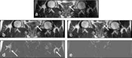
Figure 3.10: Control point selection when images are acquired with a week’s interval between them. Image (a) is from the reference volume acquired one week later with an empty bladder. Image (b) is to be warped and is from the volume acquired earlier with a full bladder. Sagittal slices best show the deformations at the bladder (vertical arrow) and rectum (horizontal arrow) where most control points are placed. Volumes are from volunteer S3.
3.3.4.5Registration Quality of Non-Rigid and Rigid Body Registration
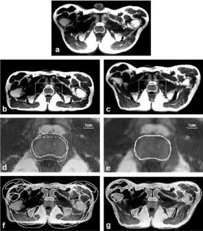
In Fig. 3.11 we compare non-rigid and rigid body registration for a typical volume pair in the treatment and diagnostic positions. Following non-rigid registration, the prostate boundary overlap is excellent (Fig. 3.11e) and probably within the manual segmentation error. Similar results were obtained in other transverse slices throughout the prostate. The prostate 3D centroid calculated from segmented images displaced by only 0.6 mm, or 0.4 voxels, following warping. Following rigid body registration, the prostate was misaligned with a displacement to the posterior of ≈3.4 mm when in the treatment position (Fig. 3.11d), as previously reported by us [1]. Using rigid body registration, there is significant misalignment throughout large regions in the pelvis (Fig. 3.11f ) that is greatly reduced with warping (Fig. 3.11g). Note that warping even allows the outer surfaces to match well. Other visualization methods such as two-color overlays and difference images, quickly show matching of structures without segmentation but do not reproduce well on a printed page.
130 |
Fei, Suri, and Wilson |
Figure 3.11: Comparison of warping and rigid body registration for volumes acquired in the treatment and diagnostic positions. Image (a) is from the reference volume acquired in the treatment position, and the prostate is manually segmented. Images in the left and right columns are from the floating volume acquired in the diagnostic position following rigid body and warping registration, respectively. To show potential mismatch, the prostate contour from the reference in (a) is copied to (b) and (c) and magnified as the dashed contours in (d) and (e). The 3 mm movement of the prostate to the posterior is corrected with warping (e) but not rigid body registration (d). Pelvic boundaries manually segmented from the reference show significant misalignment with rigid body (f ) that is greatly improved with warping (g). Images are transverse slices from subject S2.
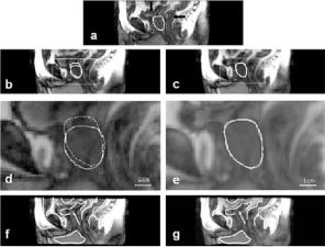
We next examine the effect of conditions such as bladder and rectal filling that might change from one imaging session to the next. In Fig. 3.12 we compare non-rigid and rigid body registration for a volume pair with one-week between imaging sessions. One volume is with an empty bladder and the other is with a relatively full bladder. There is also a difference in rectal filling. Non-rigid registration closely aligns the prostate (Fig. 3.12e) while rigid body does not
Three-Dimensional Registration Methods |
131 |
Figure 3.12: Comparison of rigid body and warping registration for volumes acquired with an interval of one week between imaging sessions. The reference image (a) with a manually segmented prostate was acquired later with an empty bladder (vertical arrow) and partial rectal filling (horizontal arrow). Images in the left and right columns are from the floating volume acquired earlier following rigid body and warping registration, respectively. To show potential mismatch, contours from the reference are shown on images following registration, as described in Fig. 3.11. The full bladder in (d) has pushed the prostate, shown by the continuous curve, in the caudal direction. After warping, prostate contours match closely (e). The bladder, rectum, and other organs closely align following warping (g). With rigid body (f ), proceeding from left to right, the front of the pelvis, the bladder (arrow), and the rectum are all misaligned. Images are sagittal slices from S3.
(Fig. 3.12d). In addition, rigid body registration does not align the bladder and parts of the rectum (Fig. 3.12f). With warping, the bladder closely matches the reference, and the rectum is better aligned (Fig. 3.12g). Other visualization methods showed excellent alignment of internal and surface edges. Difference images show that warping greatly improves alignment of internal structures as compared to rigid body registration (Fig. 3.13). The difference image following rigid body registration shows bright regions indicating misalignments (Fig. 3.13d) that are removed with warping (Fig. 3.13e).
We also examined volume pairs with both volumes acquired in the diagnostic position under comparable conditions. In the current data set, five volume
132 |
Fei, Suri, and Wilson |
Figure 3.13: Comparison of registration quality for rigid body and warping registration. The reference image (a) was acquired with a relatively empty bladder (arrow). Images (b) and (c) are from the floating volume acquired with a full bladder following rigid body and warping registration, respectively. Images (d) and (e) are the absolute difference images between the reference and registered images, respectively. Bright regions following rigid body indicate misalignments
(d) that are removed with warping (e). Images (d) and (e) are displayed using the same grayscale window and level values. Images are coronal slices from S3 volumes shown in Fig. 3.12.
pairs fit these criteria. In all such cases, rigid body registration worked as well as warping. There were no noticeable deformations in the pelvis, and prostate centroids typically displaced less than 1.0 mm between the two registered volumes. Note that this was obtained even though subjects always got up from the table and moved around before being imaged again.
3.3.4.6 Quantitative Evaluation of Non-Rigid Registration
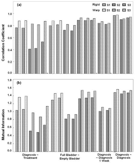
Figure 3.14 shows the correlation coefficient and mutual information values between registered volumes. Warping increased CC and MI values in every case, and a paired two-tailed t-test indicated a significant effect of warping at p < 0.5%. The most significant improvement was in the case of treatmentdiagnosis where improvements in CC and MI were as high as 102.7% and 87.8%, respectively.
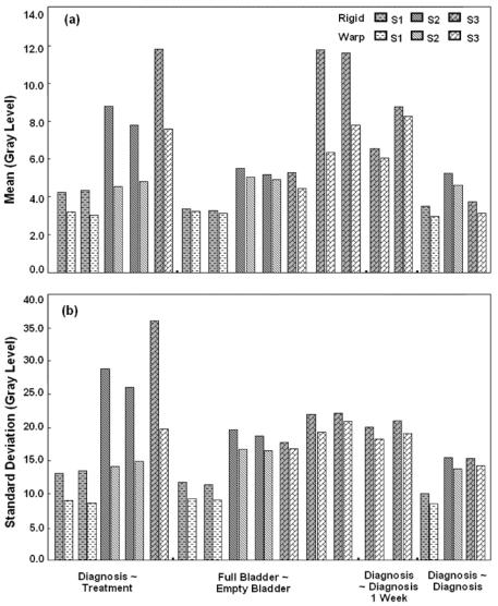
Statistics of image differences following rigid body and non-rigid registration are shown in Fig. 3.15. Warping reduces the absolute intensity difference between corresponding voxels (Fig. 3.15a), and the mean across all image volumes is only 4.2 gray levels, a value corresponding to only 4.7% of the mean image value of 90. We used the absolute intensity difference because signed
Three-Dimensional Registration Methods |
133 |
Figure 3.14: Voxel similarity measures for rigid body and warping registration. Correlation coefficient (CC) (a) and mutual information (MI) (b) following registration with (light bars) and without (dark bars) warping are plotted. Conditions described in Experimental Methods are listed on the x-axis. Warping increase CC and MI in all cases. The most significant increases occurred in the case of the treatment-diagnosis volume pairs where maximum increase in CC and MI are 101.7% and 87.8%, respectively. For volumes acquired within the same diagnostic position and comparable conditions (two right-most groups), warping did not have significant improvement over rigid body method.
134 |
Fei, Suri, and Wilson |
Figure 3.15: Image statistics of absolute intensity difference images for rigid body and warping registration. The mean (a) and standard deviation (b) are plotted. See the legend of Fig. 3.14 for other details. Warping decreased the mean and standard deviation in each case, but the most significant decreases occurred in the case of the treatment-diagnosis volume pairs. After warping, the intensity averaged over all data is 4.2 ± 1.9 gray levels, a value corresponding to only ≈4.7% of the mean image value of ≈90 gray levels.
Three-Dimensional Registration Methods |
135 |
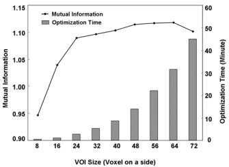
Figure 3.16: Optimization time and mutual information as a function of VOI size. The left vertical axis is mutual information, and the right vertical axis is the total VOI’s optimization time. The horizontal axis is the size of the VOI on a side. In each case, the VOI is centered on the CP, but since even numbers of voxels are used, the CP is displaced consistently to the upper left-hand corner by one voxel. With increasing VOI size, time increases linearly with the number of voxels within the VOI. The peak mutual information value is at a VOI size of 64 on a side. A treatment-diagnosis volume pair is used from S2 with 180 CPs.
values canceled when averaged over the entire image. The standard deviation of absolute difference is also reduced (Fig. 3.15b).
These quantitative measures match observation from visual inspection. For example, the third pair of the first group (diagnosis-treatment) in Figs. 15 and 16 correspond with the images in Fig. 3.11. After warping, registration greatly improved. Another interesting example is the difference images in Figs. 3.13d and 3.13e that correspond to the last pair of the second group (full-empty bladder) in Fig. 3.15. Once again, the statistical measures reflect the great change in visual quality.
3.3.4.7 Algorithmic Implementation
In rigid body registration, the multiresolution approach and restarting algorithm were important modifications. First, these two features improved robustness.
136 |
Fei, Suri, and Wilson |
The algorithm always gave very nearly the same transformation parameters (<0.01 voxels and 0.01◦) for the 17 volume pairs in this study using a wide variety of initial guesses. We also found that MI was more accurate than CC at the highest resolution [1]. Second, the multiresolution approach enabled the program to get close to the final value quickly because of the reduced number of calculations. That is, the time for reformatting at the lowest resolution of 1/4 number of voxels in a linear dimension was 0.16 minute, less than 1/63 times that at the highest resolution, a value nearly equal to the 1/64 expected from the change in the number of voxels. In a typical example, the number of restarts was 5, 1, and 1 for resolutions at 1/4, 1/2, and the full number of voxels in a linear dimension, respectively. When we checked the restarts at the resolution of 1/4 number of voxels, we determined that none of the five restarts converged to the same transformation. It has been our experience that more restarts are desirable at the lower resolutions, and the algorithm includes this feature. Each call to the Simplex optimization resulted in 50 to 100 MI evaluations before the tolerance (0.001) was reached. In some experiments on multiple volumes, we reduced the tolerance value but found little difference in registration quality, probably because of the restarting and multiresolution features. The time for rigid body registration, typically 5–10 min on a Pentium IV, 1.8 GHz CPU, with 1.0 GB of memory, could possibly be reduced to within one minute with optimized C code rather than the high level language IDL.
Some technical aspects of non-rigid registration are of interest. Fig. 3.16 shows the optimization time and MI values between registered volumes as a function of VOI size. The optimization time for 180 CPs increases roughly linearly with the number of voxels within a VOI, about 0.5 minutes for VOIs with 16 voxels on one side and 30 minutes for VOIs with 64 voxels on a side. In Fig. 3.16, the MI curve saturates at the VOI size of 64 voxels on a side which means the size of 64 gave better MI value. These curves are for the case of treatment-diagnosis for volunteer S2. When we examined the cases of full-empty bladder and volumes acquired over one week time interval, we found that the VOI size of 16 voxels on a side worked best. Using the same computer above, for a volume with 256 × 256 × 140 voxels and 180 CPs, the non-rigid registration typically takes about 15–45 minutes depending on the VOI size.
We report some details on VOI optimization for a typical treatmentdiagnosis volume pair from subject S2. Following rigid body registration, the mean distance between the manually selected reference and floating CPs was