

Kluwer - Handbook of Biomedical Image Analysis Vol
.3.pdf16 |
Farag et al. |
point in the experimental data set. This time can be significantly reduced by applying the following grid closest point (GCP) transform.
The GCP transform GCP : 3 → 3 maps each point in the 3D space G 3 that encloses the two surfaces S and S to a displacement vector, r, which represents the displacement from the closest point in the model set S. Thus for all z G
GCP(z) = r = xm − z |
(1.5) |
such that
min |
( |
z, xi |
) |
(1.6) |
||
d(z, xm) = xi |
|
S |
{d |
|
|
|
|
|
|
|
|
|
|
where d(·) is the Euclidean distance. For each point in G, the transform calculates a displacement vector to the closest point in the model data set which can be used subsequently to find matching points between S and S during the minimization process.
In the discrete case, assume that G consists of a rectangular box that encloses the two surfaces. Furthermore, assume that G is quantized into a set of L × W × H cells of size δ3
{Cijk | 0 ≤ i ≤ L , 0 ≤ j ≤ W, 0 ≤ k ≤ H} |
(1.7) |
such that
W = (Wmax − Wmin)/δ |
(1.8) |
L = (Lmax − Lmin)/δ |
(1.9) |
and
H = (Hmax − Hmin)/δ |
(1.10) |
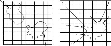
Figure 1.2 shows a 2D illustration of such a grid.
Each cell Cijk will hold a displacement vector rijk which is a vector from its centroid, denoted by c0ijk, to its closest point in the model set.
The GCP transform is applied only once at the beginning of the registration process. After its application, each cell in G has a displacement vector to its closet point in the model set. During the minimization, to calculate the closest point x˜ = C(yv , S) to a point yv S , you first have to find the intersection of yv and G. Assuming uniform quantization, the indices of the cell Cijk in which the
Medical Image Registration
Experimental Data Set S ,
δ |
δ |
Model Data Set S
17 |
rWmax,0 |
r0,0 |
Model Data Set S |
r2,Rmax |
δ |
δ |
Figure 1.2: (Left) superimposing a uniform grid G of size δ onto the space that encloses the model and experimental data sets. (Right) for each cell Cijk G, calculate a displacement rijk, from the cell centroid, c0ijk, to its closet point on S.
point yv = {u, v, w} lies can be found by
i |
= |
|
u − Lmin |
, |
j |
= |
|
v − Wmin |
, |
k |
= |
w − Hmin |
(1.11) |
|
|
|
|
δ |
|||||||||
|
|
δ |
|
|
δ |
|
|
||||||
If the content of the cell Cijk is rijk then |
|
|
|
|
|||||||||
|
|
|
|
|
x˜ = C(yv , S) = rijk + c0ijk |
(1.12) |
|||||||
An approximation of the closest point can be obtained by using the point itself instead of the centroid of the cell in which it lies
x˜ = C(yv , S) ≈ rijk + yv |
(1.13) |
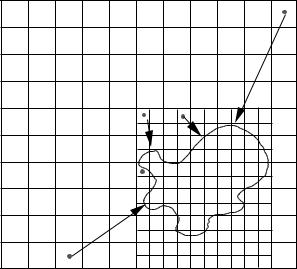
Equation (1.13) introduces an error which is a function of δ, the quantization step. This error can be reduced to some extent by using a non-uniform quantization. It should be noted that the GCP transform is spatially quantized and its accuracy depends largely on the selection of δ. The error in the displacement vector is
≤ 34 δ2. Therefore, smaller values for δ will give higher accuracy but on the extent of larger memory requirements and larger number of computations of the GCP for each cell. To solve this problem, you can select a small value for δ in the region that directly surrounds the model set, and a slightly larger value (in this work 2δ) for the rest of the space G. This enables a coarse matching process
18 |
Farag et al. |
at the beginning of the registration and fine matching toward the end of the minimization.
The next step is to search for the transformation parameters using genetic algorithms (GAs). GAs, pioneered by Holland [23], are adaptive, domain independent search procedures derived from the principles of natural population genetics. GAs borrow its name from the natural genetic system. In natural genetic system whether a living cell will perform a specific and useful task in a predictable and controlled way is determined by its genetic makeup, i.e., by the instructions contained in a collection of chemical messages called genes [24]. Genetic algorithms are briefly characterized by three main concepts: a Darwinian notion of fitness or strength which determines an individual’s likelihood of affecting future generations through reproduction; a reproduction operation which selects individuals for recombination to their fitness or strength; and a recombination operation which creates new offspring based on the genetic structure of their parents.
Genetic algorithms work with a coding of a parameter set, not the parameters themselves and search from a population of points, not a single point. Also genetic algorithms use payoff (objective function) information, not derivatives or other auxiliary knowledge and use probabilistic transition rules, not deterministic ones. These four differences contribute to genetic algorithms’ robustness and resulting advantage over other more commonly used search and optimization techniques (see Fig. 1.3).
Since the genetic algorithm works by maximizing an objective function, the fitness function, Fr (R, t), can be defined as in Eq. (1.3).
Combining (1.3) with the GCP transform to find matching points between the two data sets, Eq. (1.3) can be rewritten as
n
Fr (R, t) = − d2(y , GCP(yi) + yi) |
(1.14) |
i=1 |
|
where yi = Ryi + t. By maximizing (1.14) we effectively minimize (1.3).
The objective of the registration process is to obtain the rotation matrix R and the translation vector t. Thus in 3D space, there are six parameters that need to be evaluated; the three angles of rotation around the three principal axes α, β, and γ , and the displacement x, y, and z in the x, y, z directions, respectively.
Medical Image Registration |
19 |
rWmax,0
|
δ/2 |
|
r2,Rmax |
δ |
|
δ |
δ/2 |
Figure 1.3: An example of a non-uniform grid G.
In the 2D space, the parameter set is reduced to x, y, and the angle of rotation θ . These parameters are represented by binary notation to minimize as much as possible the length of the schemata d(H) and the order of the schemata
O (H). The number of bits np, assigned to each parameter, p, depends on the type of application and the required degree of accuracy. The number of bits should be chosen as small as possible to minimize the time of convergence of the genetic algorithm. For example, you can assign 8 bits each, thus allowing a displacement of ±127 units. A range of ±31 can also enforced over the angles of rotation. Therefore 6 bits are assigned for each angle of rotation. As shown in Fig. 1.4, the genes are formed from the concatenation of the binary coded parameters.
The selection operator chooses the highest fitted genes for mating using a Roulette wheel selection [24]. The crossover and mutation operators are implemented by choosing a random crossover and mutation point with probabilities
Pcp and Pmp, respectively, for each coded parameter p. The generated strings are concatenated together to form one string from which the populations are formed (see Fig. 1.5).
More details and error analysis of the GCP technique can be found in [9]. The major drawback of the GCP/GA algorithm is that the range of the transformation
20 |
|
|
|
|
|
|
|
|
|
|
|
|
|
|
|
|
|
|
|
|
|
|
|
|
|
|
|
|
|
|
|
|
|
|
|
|
|
|
|
|
|
|
|
|
|
|
|
|
|
|
|
|
|
Farag et al. |
||
|
|
Population |
|
|
|
|
|
|
|
|
|
|
|
|
|
|
|
|
|
|
|
|
|
|
|
|
|
|
|
|
|
|
|
|
|
|
|
|
|
|
|
|
|
|
||||||||||||
|
|
|
|
|
|
|
|
|
|
|
|
|
|
|
Displacements |
|
|
|
|
|
|
|
|
Rotations |
|
|
|
|
|
|||||||||||||||||||||||||||
|
|
|
|
|
|
|
|
|
|
|
|
|
|
|
|
|
|
|
|
|
|
|
|
|
|
|
||||||||||||||||||||||||||||||
|
|
|
|
|
|
|
|
|
|
|
|
|
|
|
|
|
|
|
|
|
|
|
|
|
|
|
|
|||||||||||||||||||||||||||||
|
|
|
|
|
|
|
|
|
|
|
|
|
|
|
|
|
|
|
|
|
|
|
|
|
|
|
|
|
|
|
|
|
|
|
|
|
|
|
|
|
|
|
|
|
|
|
|
|
|
|
|
|
|
|
|
|
|
|
|
|
|
|
|
|
|
|
|
∆ x |
|
|
|
∆y |
|
|
|
|
|
|
∆ z |
|
|
α |
|
|
|
|
β |
|
|
γ |
|
|
|||||||||||||||||||||
|
|
|
|
|
|
|
|
|
|
|
|
|
|
|
|
|
|
|||||||||||||||||||||||||||||||||||||||
|
|
|
|
|
|
|
|
|
|
|
|
|
|
|
|
|
|
|||||||||||||||||||||||||||||||||||||||
|
|
|
|
|
|
|
|
|
|
|
|
8b |
|
|
|
|
|
8b |
|
|
|
|
|
|
|
|
8b |
|
|
|
|
|
|
6b |
|
|
|
|
|
|
|
6b |
|
|
|
|
|
|
6b |
|
|
|
||||
|
|
|
|
|
|
|
|
|
|
|
|
|
|
|
|
|
|
|
|
|
(a) |
|
|
|
|
|
|
|
|
|
|
|
|
|
|
|
|
|
|
|
|
|
|
|
||||||||||||
|
|
|
|
|
|
|
|
|
|
|
|
|
|
|
|
|
|
|
|
|
|
|
|
|
|
|
|
|
|
|
|
|
|
|
|
|
|
|
|
|
|
|
|
|||||||||||||
|
|
|
|
|
|
|
|
|
|
|
|
|
|
Displacements |
|
Rotation |
|
|
|
|
|
|||||||||||||||||||||||||||||||||||
|
|
|
|
|
|
|
|
|
|
|
|
|
∆ x |
|
|
|
∆y |
|
|
|
θ |
|
|
|
|
|
|
|
|
|
|
|
|
|
|
|
|
|||||||||||||||||||
|
|
|
|
|
|
|
|
|
|
|
|
|
|
|
|
|
|
|
|
|
|
|
|
|
|
|
|
|
||||||||||||||||||||||||||||
|
|
|
|
|
|
|
|
|
|
|
|
|
|
|
|
|
|
|
|
|
|
|
|
|
|
|
|
|
||||||||||||||||||||||||||||
|
|
|
|
|
|
|
|
|
|
|
|
|
|
|
|
|
|
|
|
|
|
|
|
|
|
|
|
|
|
|
|
|
|
|
|
|
|
|
|
|
|
|
|
|
|
|
|
|
|
|
|
|
|
|
|
|

 8b
8b 

 8b
8b 

 6b
6b
(b)
Figure 1.4: Different gene structures.
Generations |
1 |
|
|
gene 1 |
|
gene 1 |
|
|
fit. 5% |
|
|
gene 2 |
|
gene 2 |
|
. |
fit. 1% |
. |
|
. |
. |
||
|
|||
. |
|
. |
|
gene 25 |
|
gene 25 |
|
. |
|
. |
|
. |
fit. 2% |
. |
|
. |
. |
||
|
2
. . .
gene 1
fit. 7%
gene 2
fit. 10%
gene 25
.
fit. 9% .
.
5
. . .
gene 1
fit. 25%
|
gene 2 |
|
. |
fit. 60% |
. |
|
. |
gene 25
|
. |
|
fit. 98% |
. |
|
. |
||
|
50
fit. 95%
fit. 97%
fit. 99%
gene 100 |
gene 100 |
gene 100 |
|
gene 100 |
|
fit. 7% |
fit. 0.5% |
fit. 40% |
fit. 95% |
Figure 1.5: An illustration of the GA use in calculating the transformation parameters. The process starts by coding the transformation parameters into one string. An initial population of strings is randomly generated. Applying the selection, crossover and the mutation operations, new generations are obtained. Notice how the registration fitness function average increases with the generations. Maximum fitness can be reached eventually.
Medical Image Registration |
21 |
parameters needed to be known beforehand to efficiently code them into a string. Also if the range is large, the GA convergence can be slow.
1.5 Feature-Based Registration Techniques
Feature-based registration techniques rely on extracting and matching similar features vector between two or more data sets in order to find corresponding data points. So the two critical procedures involved in feature-based registration is feature extraction and feature correspondence. Feature representations, which are invariant to scaling, rotation, and translation, are more desirable in the matching process.
One of the most successful feature-based registration techniques, especially for multimodal registration, is by maximization of mutual information
(MI) [25]. This technique works well for both MR and CT since they are informative of the same underlying anatomy and there will be mutual information between the MR image and the CT image. Such a technique would attempt to find the registration by maximizing the information that one volumetric image provides about the other. It requires no a priori model of the relationship between the modalities, it only assumes that one volume provides the most information about the other one when they are correctly registered.
Unfortunately, if initial transformation between the two modalities is unknown, the MI will converge slowly. So, we will demonstrate how to use a composite registration procedure that integrates another feature-based registration technique, mainly a surface-based [26] registration technique, to estimate the initial transformation. Surface-based registration techniques use features available on the data set surface mesh such as density or curvature. The surfacebased registration techniques work better for free-form surfaces, such as the skin contours, while MI works better for voxel-based volumes. Such composite registration procedures have become recently the state-of-the-art in most registration applications due to the fact that most feature-based techniques are complementary in nature.
1.5.1 Surface-Based Registration Algorithm
In order for any surface-based registration algorithm to perform accurately and efficiently, an appropriate representation scheme for the surface is needed.
22 |
Farag et al. |
Most of the surface representation schemes found in literature have adopted some form of shape parameterization especially for the purpose of object recognition. However, free-form surfaces, in general (e.g., CT/MRI skin contours), may not have simple volumetric shapes that can be expressed in terms of parametric primitives. Some representation schemes for free-form surfaces found in literature include the “splash” representation proposed by Stein and Medioni [27] in which the surface curvature along the intersection of the surface and a sphere centered at the point of interest is calculated for different sphere diameters and a signature curve is obtained for this point. Also the work of Chua and Jarvis [28], who proposed the “point signature” representation which describes the local underlying surface structure in the neighborhood of a point. This is obtained by plotting the distance profile of a circle of points to a plane defined by that circle of points. Dorai and Jain [29] proposed another representation called “COSMOS” for free-form objects in which an object is described in terms of maximal surface patches of constant shape index from which properties such as surface area, curvedness and connectivity are built into the representation. Johnson and Hebert [30] recently introduced a new representation scheme called the “spin image”. This image represents the histogram of the surface points relative to a certain oriented point. This image is generated for each oriented point on the surface and matching between two surfaces is done by matching the spin images of the points in the two surfaces. Yamany and Farag [26] introduced another technique based on surface signatures. Surface signatures are 2D images formed by coding the 3D curvature information seen from a local point. These images are invariant to most transformation. In what follows are some details for some of these algorithms.
1.5.1.1 The “Splash” Surface Registration
Geometric indexing have been one of the most used surface indexing techniques because it used the geometrical relationships between invariant features. However, another form of indexing that uses local shape information has become more popular. As it is based on structural information local to the neighborhood of a point, this indexing method is called “Structural indexing”.
Circle of points was first used to describe the underlying surface structure around a given point. This can be done by decomposing the local surface patch
Medical Image Registration |
23 |
R
AVERAGE NORMALS
R
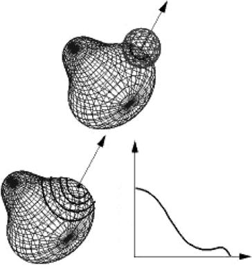
Figure 1.6: An illustration of the “splash” representation scheme. At specific points on the surface, the intersections of the surface patches and the spheres of prefixed radii are obtained. For each intersection a curve representing the average normal of the points in the intersection and the point in study is obtained. These curves are further used for matching.
around a specific point into a series of contours, each of which is the locus of all points at a certain distance from the specific point.
Stein and Medioni [27] extended this idea further. Instead of decomposing a surface patch into a series of contours of different radii, a few contours at prefixed radii are extracted as shown in Fig. 1.6. On each contour of points, surface normals are computed. This contour is called a “splash”. A 3D curve is constructed from the relationship between the splash and the normal at the center point. This curve is converted into piecewise linear segments. Curvature angles between these segments and torsion angles between their binormals are computed. These two features are used to encode the contour.
24 |
Farag et al. |
Matching is performed using the contour codes of points on the two surfaces. Fast indexing was achieved by hashing the codes for all models in the library into an index table.
At runtime recognition, the splashes of highly structured regions are computed and encoded using the same encoding scheme. Models which contain similar codes as the splashes appearing in the scene are extracted. Verification is then performed for each combination of three correspondences.
1.5.1.2 The “Point Signature” Surface Registration
This approach was introduced by Chua and Jarvis [28] for fast recognition. They establish a “signature” for each of the given 3D data points rather than just depending on the 3D coordinates of the point. This is similar to the “splash” representation but instead of using the relationship between the surface normals of the center points and its surrounding neighbors, they used the point set itself.
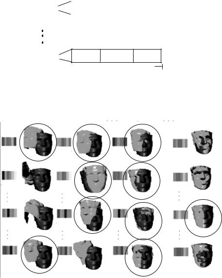
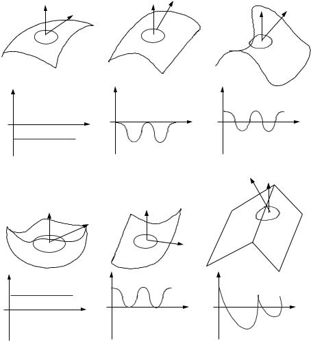
For a given point p, they place a sphere of radius r, centered at p (similar to the method used in splash as depicted in Fig. 1.6). The intersection of the sphere with the object surface is a 3D space curve whose orientation can be defined by a directional frame formed of the normal to the plane fitted to the curve, a reference direction and their cross product. The next step is to sample the points on this curve starting from the reference direction. For each sampled point there exist two information, the distance from itself to the fitted plane and the clockwise angle about the normal from the reference direction. Figure 1.7 shows some typical examples of point signatures for different surface types.
Due to this simple representation, the 3D surface matching is transformed into 1D signature matching. In their paper they analyze this signature matching and estimate the accepted error tolerance in the matched signature. Prior to recognition, the model library is built by computing the point signatures for each point in the model and for every model. They also used hashing to index the signatures in a table. At runtime, the surface under study is sampled at a fixed interval and the sampled points are used in the matching process.
1.5.1.3 The “COSMOS” Surface Registration
The goals of the COSMOS (Curvedness-Orientation-Shape Map On Sphere) representation scheme were, first, to be a general representation scheme that can
Medical Image Registration
N
Ref
d |
d |
|
θ
(a)
N
Ref
25
N |
Ref |
N |
|
||
|
|
Ref
|
d |
|
θ |
|
θ |
(b) |
|
(c) |
|
Ref |
N |
|
|
N
Ref
d |
d |
d |
|
|
|
θ |
θ |
θ |
(d) |
(e) |
(f ) |
Figure 1.7: Examples of point signatures: (a) peak, (b) ridge, (c) saddle, (d) pit, (e) valley, (f) roof edge.
be used to describe sculpted objects, as well as objects composed of simple analytical surface primitives. Second, to be as compact and as expressive as possible for accurate recognition of objects from single range image.
The representation uses the “shape index” to represent complex objects. An object is characterized by a set of maximally sized surface patches of constant shape index and their orientation dependent mapping onto the unit sphere.