

Kluwer - Handbook of Biomedical Image Analysis Vol
.3.pdf6 |
Farag et al. |
flexible, yet more complex and the methods range from using cross correlation, variance minimization, histogram clustering and the famous maximization of mutual information (discussed later in details).
1.2.3 Nature of Transformation
Since the registration process tries to recover the optimal transformation between two candidate subjects, the nature of such transformation categorize the registration procedure to be used. The most commonly used is the rigid registration where the transformation involves only translations and rotations. If the transformation maps parallel lines onto parallel lines it is called affine. If it maps lines onto lines, it is called projective. Finally, if it maps lines onto curves, it is called curved or elastic. Each type of transformation contains as special cases the ones described before it, e.g., the rigid transformation is a special kind of affine transformation. A composition of more than one transformation can be categorized as a single transformation of the most complex type in the composition, e.g., a composition of a projective and an affine transformation is a projective transformation, and a composition of rigid transformations is again a rigid transformation. Also a transformation is called global if it applies to the entire image, and local if subsections of the image each have their own transformations defined.
Rigid and affine transformations are generally global, and curved transformations are local. This is due to the physical model underlying the curved transformation type. Affine transformations are typically used in instances of rigid body movement where the image scaling factors are unknown or suspected to be incorrect, such as in MRI images due to geometric distortions. The projective transformation type has no real physical basis in image registration except for 2D/3D registration, but is sometimes used as a constrained-elastic transformation when a fully elastic transformation behaves inadequately or has too many parameters to solve.
1.2.4 Interaction
Three levels of interaction can be involved in registration procedures. Automatic, where the user only supplies the algorithm with the image data and possibly information on the image acquisition. Interactive, where the user does the
Medical Image Registration |
7 |
registration himself, assisted by software supplying a visual or numerical impression of the current transformation, and possibly an initial transformation guess.
Semi-automatic, where the interaction required can be of two different natures: the user needs to initialize the algorithm, e.g., by segmenting the data, or steer the algorithm, e.g., by rejecting or accepting suggested registration hypotheses.
1.2.5 Optimization Procedure
There exists two possible ways of finding the transformation parameters. Either they are computed directly from the available image information, or they are looked for based on a certain optimization criterion. Many applications use more than one optimization technique, frequently a fast but coarse technique followed by an accurate yet slow one (as shown later).
1.2.6 Modalities Involved
Four classes of registration tasks can be recognized based on the modalities that are involved. In monomodal applications, the images to be registered belong to the same modality, as opposed to multimodal registration tasks, where the images to be registered stem from two different modalities. The other two are modality to model and model to modality registration where only one image is involved and the other modality is either a model or the patient himself. The model to modality is used frequently in intraoperative registration techniques. Monomodal tasks are well suited for growth monitoring, intervention verification, rest-stress comparisons, ictal-interictal comparisons, subtraction imaging (also DSA, CTA), and many other applications. The applications of multimodal registration are abundant and diverse, predominantly diagnostic in nature. A coarse division would be into anatomical-anatomical registration, where images showing different aspects of tissue morphology are combined, and functionalanatomical, where tissue metabolism and its spatial location relative to anatomical structures are related.
1.2.7 Subject
There can be intrasubject registration involving images for the same patient, intersubject registration involving images for different patients and atlas
8 |
Farag et al. |
registration where one image is acquired from a single patient, and the other image is somehow constructed from an image information database obtained using imaging of many subjects.
1.3 General Registration Theory
In general, registration is the process by which two or more data sets are brought into alignment. Registration can be defined as “the process of finding a set of transformation operations between two or more data sets such that the overlap between these sets in a certain common space minimizes a certain optimization criterion”.
The registration problem can be mathematically represented as follows:
A parametric shape S, either a curve segment or a surface, is a vector function,
x : [a, b] → 3 |
(1.1) |
for curves where a and b are scalars and
x : 2 → 3 |
(1.2) |
for surfaces. Both curve and surface data sets are usually in the form of, or can be easily converted to, a set of 2D or 3D points, which represent the most general form of 2D or 3D curves and surfaces including free-from curves and surfaces. Let the points in the first, or model data set, S, be denoted by {xi|i = 1, . . . , m}, and those in the second, or experimental data set, S , be denoted by {y j | j =
1, . . . , n}. We want to find a transformation matrix T such that when applied to
S , the distance from each point on the resulting surface and its corresponding point on the model surface S is zero in the noise free case.
For the case of rigid registration (without considering the scaling factor), the transformation matrix T consists of two components: a rotation matrix R, and a translation vector t. The objective of registration is to determine R and t such that the following criterion is minimized
n
F(R, t) = d2(Ryi + t, S). |
(1.3) |
i=1 |
|
where d(yi, S) denotes the distance of point yi to shape S.
If we add the scaling factor as a third component, then the matrix T represents a matrix called the similarity transformation matrix. In this case the
Medical Image Registration |
9 |
new shape will be similar to the original shape but at a different scale. It should be noticed that we will use the term similarity transformation to represent a rotation, translation and scaling only, no shear or torsion or other deformable transformations are included.
The minimization of Eq. (1.3) is very difficult because d(Ryi + t, S) is highly nonlinear since the correspondence between yi and S is not known beforehand.
To understand the challenges involved in solving the registration problem one needs to understand the following:
1.For two data sets, if the transformation from one to the other is precisely known, then the registration process would be trivial. But when the transformation is only approximately known, the problem becomes more difficult. It is here that most researchers have addressed this problem. However, few researchers have attempted to solve the problem when the transformation is totally unknown.
2.The search for an unknown, optimal transformation invariably assumes an initial transformation which is iteratively refined through the minimization of some evaluation function. Such search may lead to a local minimum and, unless a global optimizer is used [3], it is difficult to reach a global solution.
3.For many applications (e.g., intraoperative registration), the registration time can be very critical and near real-time registration process is still needed.
The registration process must compensate for three very important problems, which are translational offset, rotational misalignment, and partial data sets. Error due to translational offset occurs when the coordinate origins of the data sets are not the same point in N-dimensional space. This can be demonstrated by calculating the point by point error of two identical surfaces located at different locations in the N-dimensional space. Even though the data sets are identical, the average experimental data error will be equal to the distance of the offset between the two sets.
Registration must also correct for error due to rotational misalignment between the data sets. This can be visualized by viewing a non-symmetrical surface from two different angles. The two different views may appear very different even though they come from the same surface. Once the views are rotated into correct alignment, an accurate value for the error measure can be obtained.
10 |
Farag et al. |
The last major problem that the registration process must address is aligning data sets that represents only a portion of the model data. A correspondence between the experimental data set and the corresponding portion of the model data set must be established before correcting for translation and rotation errors. Once this is accomplished, the error measure must be calculated for only the overlapping portions of the two sets. For example, consider scanning a tooth and attempting to calculate the error between the scanned tooth and a model of an entire human jaw. The registration process must be able to determine which region of the jaw coincides with the scanned tooth, assuming the tooth is distinct enough to distinguish between the other teeth, and then calculate the error measure using only the overlapping regions.
In terms of algorithmic implementations, all of the registration techniques fall under two global implementation categories: distance-based and featurebased approaches. In the distance-based approach, the goal is to calculate the transformation by minimizing a criterion relating the distance between the two data sets. In the feature-based approach some differential properties invariant to rigid transformation (such as gray level value, histogram, curvature, mutual information, entropy, etc.) are often used.
In the following sections we will discuss in some details examples of algorithms in both the approaches.
1.4 Distance-based Registration Techniques
Among the distance-based techniques, Besl and McKay [4] proposed the Iterative Closest Point (ICP) algorithm which establishes correspondences between data sets by matching points in one data set to the closest points in the other data set. ICP is an elegant way to register different data sets because it is intuitive and simple. Besl and McKay’s algorithm requires an initial transformation that places the two data sets in approximate registration and operates under the condition that one data set be a proper subset of the other. Since their algorithm looks for a corresponding scene point for every model point, incorrect registration can occur when a model point does not have a corresponding scene point due to occlusion in the scene. Attempts at solving these problems have led to several variants of the original algorithm.
The ICP algorithm matches points in the experimental data set after applying the previously recovered transformation (R, t), where R is a matrix represent-
Medical Image Registration |
11 |
ing the rotation transformation and t is a vector representing the translation transformation, with their closest points in the model data set. A least-squares estimation is then used to reduce the average distance between the matched points in the two data sets. The algorithm is relatively straightforward and can be summarized as follows:
1.Given a motion transformation that initially aligns two data sets to some degree, a set of correspondence is developed between the points in each set. This is done using a simple metric: for each point in the first data set, pick the point in the second set which is closest to it under the current transformation.
2.From this set of correspondence an incremental motion can be computed which further aligns these points to one another.
3.Those two steps are iterated until some convergence criterion is satisfied.
Figure 1.1 illustrates these steps. The ICP algorithm tries to find the optimal transformation matrix T between two shapes S and S such that Eq. (1.3) is minimized using the closest point operator in distance calculations as follows:
d(yi, S) = ||yi − C(yi, S)|| |
(1.4) |
where C(·) is defined as the closest point operator, i.e., C(·) finds the closest point in shape S to the point yi. At each step of the minimization process, a correspondent point on S has to be found for each point Ryi + t on S . This makes the operation of registration of order O (mn) and as a result ICP has many drawbacks:
1.One of the main disadvantages of the ICP algorithm is its computation complexity. This makes the algorithm not suitable for applications where near real-time performance is required.
2.The algorithm converges successfully to a local solution but there is no guarantee that it will reach a global solution.
3.Proper convergence only occurs if one of the data sets is a subset of the other. The presence of points in each set that are not in the other leads to incorrect correspondences, which subsequently generates nonoptimal transformations.
12 |
Farag et al. |
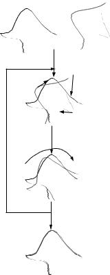
The initial two surfaces
1– Initial alignment
2– Find correspondence between closest points
3– Calculate an incremental motion
4– Iterate until some convergence criterion is satisfied
Figure 1.1: A diagram illustrating the distance-based registration algorithm steps which start by an initial alignment and then finding correspondence from which incremental motion is calculated and this process iterates until convergence.
Attempts at solving these problems have led to several variants of the original algorithm. In what follows, we provide a review of these improvements. Another good review can be found in [5].
1.4.1 Improving Correspondence
The first improvement to the basic algorithm changes the simple point-to-point correspondence used in many of the methods [4, 6, 7, 8, 9] to that between a point and a location on the surface represented by the other data set. This potentially increases the integration accuracy beyond that of the sampling resolution.
Medical Image Registration |
13 |
The first such effort was by Chen and Medioni [7]. They have improved the ICP algorithm by minimizing the distance from the sensed point to the nearest estimated plane approximating the model surface. They begin by finding the data point in the second set that is closest to a line through the point in the first set in the direction of its estimated surface normal. Then the tangent plane at this intersection point is used as the surface approximation. Yet finding the estimated plane involves another iterative procedure which further adds to the computation complexity. They reduced the complexity by selecting some important points on the smooth surfaces of the object and used these points for the registration. This works well if the smooth surfaces are uniformly distributed over the object, which is not the case for many free-form objects. More accurate but time-consuming estimates of the surface have also been used, such as octrees [10], triangular meshes [11], and parametric surfaces [12].
Most researchers have used, the simple Euclidean distance in determining the closest point [3, 4, 6, 7, 8, 9, 11, 12, 13, 14]. Fewer have used higher dimensional feature vectors, such as including the estimated surface normal [15].
1.4.2 Thresholding Outliers
Most of the early algorithms were limited by the original assumption that one data set was a subset of the other [4, 7, 8, 11, 12, 14]. Proposals to bypass this limitation have involved imposing a heuristic threshold on either the distance allowed between points in a valid pairing [6, 9, 10, 13, 15] and the deviation of the surface normals of corresponding points [15]. Any point pairs which exceed these thresholds or constrains are assumed to be incorrect. These thresholds are usually predefined constants related to the estimated accuracy of the initial transformations and can be difficult to choose robustly. Dynamically adjustable thresholds have been based on both the distribution of the distance errors at each iteration [6] and a fuzzy set classification of inlier and outliers correspondences [16].
1.4.3 Computational Requirements
In all of the techniques, computing potential correspondences is generally the most time-consuming step. In a brute-force approach [4, 15, 12], an O (N2) number of comparisons is performed to find N pairings. One way to reduce
14 |
Farag et al. |
the actual time, with a potential loss of accuracy [11], is to subsample the original data sets. Criteria for sub-sampling include taking a simple fraction of the original number [13], using multiple scales of increasing resolution [3], or taking points in areas away from surface discontinuities [7], in areas of fine detail [8], and in small random sets for robust transform estimation [14]. A more accurate and slower alternative is to use the full original data sets, but organize the closest point search using efficient data structures such as the octree [10] and k-d tree [6]. The k-d tree is even more efficient, O (NlogN), when higher order features of the points are incorporated in the distance metric.
1.4.4 Computing Intermediate Motions
Once a set of correspondences has been determined, a motion transform must be computed that best aligns the points. The most common approach is to use one of several least squares techniques to minimize the distances between corresponding points [4, 6, 8, 11, 14, 7]. In certain cases [6], individual point contributions are weighted based on the suspected noise of different portions of the data sets. More robust estimation using the least median squares technique (clustering many transforms computed from smaller sets of points) has been tried by Masuda et al. [14]. Alternatively, a Kalman filter has been used to track the intermediate motion at each iteration as new correspondences are computed [6]. More involved techniques compute the motion transform via some form of search in the space of possible transforms, trying to minimize a cost function such as the sum of distance errors across all corresponding points. Movements in transform parameter space are computed based on the changing nature of the function. Such standard search strategies as Levenberg-Marquardt [10, 12], simulated annealing [13] and genetic algorithms [9] have been used. Correspondences must be periodically updated during the search to keep the error function current. Updating too frequently can drastically increase the amount of computation, while too few updates can lead to an incorrect minimization.
1.4.5 Initialization and Convergence of Searches
As mentioned earlier, an ICP-based refinement occurs after some initial set of transformations has been determined. Some researchers assume that this
Medical Image Registration |
15 |
estimate is determined by a previous process [6, 7, 11, 12, 14], possibly calculated using feature sets. Other prior estimates can be given by a rotary table [10], a robot arm [13], or even the user. Most such estimates are assumed to be quite accurate so that using one of the various distance thresholds during matching will prune outliers correctly. Other researchers do their own featurebased alignment prior to refinement using such characteristics as principal moments [4] or similar triangles on a mesh representation of the data [8]. If these distinguishing features are absent, a uniform distribution of starting points can always be processed [4]. All of the ICP algorithms must use some set of criteria to detect convergence of the final transformation. For those techniques that compute intermediate motions using least squares methods, convergence is achieved when the transform implies a sufficiently small amount of motion [6, 8, 14] or the distance between corresponding points becomes suitably close [4, 7, 11, 14]. The iterative searches of parameter space typically converge based on small changes in the parameters or error value, or if the shape of the cost function at the current value indicates a function minimum. Any method can be terminated if convergence is not detected after some maximal number of iterations [3].
1.4.6 A Genetic Distance-based Technique
Another enhancements on the ICP algorithm for fast registration of two sets of 3D curves or surfaces was done by applying a distance transform to the model surface [3, 9]. The distance transform essentially converts the 3D space surrounding the two data sets into a field in which every point stores the magnitude and direction of a displacement vector from this point to the nearest surface element. Thus the cost function is largely precomputed. Such a transform is called the grid closest point (GCP) [9]. A genetic algorithm (GA) is then used to minimize the cost function.
Genetic algorithms (GAs) [17] provide a powerful and domain-independent search method for complex, poorly understood search spaces. Genetic algorithms have been applied to a wide diversity of problems such as combinatorial optimization [18], VLSI layout [19], machine learning [20], scene recognition [21], and adaptive image segmentation [22].
As mentioned in the previous section, to perform registration most of the computation time is spent in finding the closest point in the model set to every