

Kluwer - Handbook of Biomedical Image Analysis Vol
.3.pdfChapter 6
Inverse Consistent Image Registration
G. E. Christensen1
6.1 Introduction
Image registration has many uses in medicine such as multimodality fusion, image segmentation, deformable atlas registration, functional brain mapping, image guided surgery, and characterization of normal vs. abnormal anatomical shape and variation. The fundamental assumption in each of these applications is that image registration can be used to define a meaningful correspondence mapping between anatomical images collected from imaging devices such as CT, MRI, cryosectioning, etc. It is often assumed that this correspondence mapping or transformation is one-to-one, i.e., each point in image T is mapped to only one point in image S and vice versa. A fundamental problem with a large class of image registration techniques is that the estimated transformation from image T to S does not equal the inverse of the estimated transform from S to T. This inconsistency is a result of the matching criteria’s inability to uniquely describe the correspondences between two images. Inverse consistent registration seeks to overcome this limitation by jointly estimating the transformation from T to S and from S to T while minimizing the correspondence inconsistencies between the forward and reverse transformations. Forward and reverse transformations that are inverses of each other are defined to be inverse consistent with each other. The inverse consistency error is a measure of the difference between the forward transformation and the inverse of the reverse transformation, and vica versa.
1 Department of Electrical and Computer Engineering, The University of Iowa, Iowa City,
IA 52242 USA
219
220 |
|
Christensen |
T(x) |
h(x) |
S(x) |
|
|
g(x)
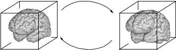
Figure 6.1: Consistent image registration is based on the principle that the mappings h from T to S and g from S to T define a point by point correspondence between T and S that are consistent with each other. This consistency is enforced mathematically by jointly estimating h and g while minimizing the inverse consistency error (||h − g−1|| + ||g − h−1||). The inverse consistency error is minimized when h and g are inverse mappings of one another.
The forward transformation h from image T to S and the reverse transformation g from S to T are pictured in Fig. 6.1. Ideally, the transformations h and g should be uniquely determined and should be inverses of one another provided the images only differ in shape and not structure. Estimating h and g independently very rarely results in a consistent set of transformations due to a large number of local minima. To overcome this deficiency in current registration systems, we jointly estimate h and g while minimizing the inverse consistency error defined as ||h − g−1|| + ||g − h−1||. Notice that the inverse consistency error is minimized when the transformations h and g are inverse mappings of one another. Jointly estimating the forward and reverse transformations provides additional correspondence information and helps ensure that these transformations define a consistent correspondence between the images. Although uniqueness is very difficult to achieve in medical image registration, the joint estimation should lead to more consistent and biologically meaningful results since information from one registration direction minimizes registration ambiguities in the other direction.
Image registration algorithms use landmarks [1–4], contours [5–7], surfaces [8–11], volumes [6, 12–21], or a combination of these features [22] to manually, semi-automatically or automatically define correspondences between two images. The need to impose the invertibility consistency constraint depends on the particular application and on the correspondence model used for registration. In general, registration techniques that do not uniquely determine the correspondence between image volumes should benefit from the consistency constraint.
Inverse Consistent Image Registration |
221 |
This is because such techniques often rely on minimize/maximize a similarity measure which has a large number of local minima/maxima due to the correspondence ambiguity. Examples include methods that minimizing/maximizing similarity measures between features in the source and target images such as image intensities, object boundaries/surfaces, etc. In theory, the higher the dimension of the transformation the more local minima these similarity measures have. Methods that use specified correspondences for registration will benefit less or not at all from the invertibility consistency constraint. For example, landmark based registration methods implicitly impose an invertibility constraint at the landmarks because the correspondence defined between landmarks is the same for estimating the forward and reverse transformations. However, the drawbacks of specifying correspondences include requiring user interaction to specify landmarks, unique correspondences can not always be specified, and such methods usually only provide coarse registration due to the small number of correspondences specified.
In this chapter, we will restrict our analysis to the class of applications that can be solved using diffeomorphic transformations. A diffeomorphic transformation is defined to be continuous, one-to-one, onto, and differentiable. The diffeomorphic restriction is valid for a large number of problems in which the two images have the same structures and neighborhood relationships but have different shapes.
Diffeomorphic transformations maintain the topology and guarantee that connected subregions of an image remain connected, neighborhood relationships between structures are preserved, and surfaces are mapped to surfaces. Preserving topology is important for synthesizing individualized electronic atlases the knowledge base of the atlas maybe transferred to the target anatomy through the topology preserving transformation providing automatic labeling and segmentation. If the total volume of a nucleus, ventricle, or cortical subregion are an important statistic it can be generated automatically. Topology preserving transformations that map the template to the target can also be used to study the physical properties of the target anatomy such as mean shape and variation. Likewise, preserving topology allows data from multiple individuals to be mapped to a standard atlas coordinate space [23]. Registration to an atlas removes individual anatomical variation and allows information from many experiments to be combined and associated with a single canonical anatomy.
222 |
Christensen |
Other investigators have proposed methods for enforcing pairwise consistent transformations. For example, Woods et al. [24] computes all pairwise registrations of a population of image volumes using a linear transformation model, i.e., a 3 × 3 matrix transformation. They then average the transformation from
Tto S with all the transformations from T to X to S. The original transformation from T to S is replaced with average transformation. The procedure is repeated for all the image pairs until convergence. This technique is limited by the fact that it can not be applied to two data sets. Also, there is no guarantee that the generated set of consistent transformations are valid. For example, a poorly registered pair of images can adversely affect all of the pairwise transformations.
The method described in this chapter is most similar to the approach described by Thirion [6]. Thirion’s idea was to iteratively estimate the forward h, reverse g, and residual r = h ◦ g transformations in order to register the images
Tand S. At each iteration, half of the residual r is added to h and half of the residual r is mapped through h and added to g. After performing this operation, h ◦ g is close to the identity transformation. The advantage of Thirion’s method is that it enforces the inverse consistency constraint without having to explicitly compute the inverse transformations as in Eq. (6.2). The residual method is an approximation to the inverse consistency method in that the residual method approximates the correspondences between the forward and reverse transformations while the inverse consistency method computes those correspondences. Thus, the residual approach only works under a small deformation assumption since the residual is computed between points that do not correspond to one another. This drawback limits the residual approach to small deformations and it therefore can not be extended to nonlinear transformation models. On the other hand, the approach presented in this paper can be extended to the nonlinear case by modifying the procedure used to calculate the inverse transformation to include nonlinear transformations.
6.2 Inverse Consitent Image Registration
6.2.1 Problem Statement
Assume that T and S correspond to two continuous images defined on the co-
ordinate system = [0, 1)3. Traditionally, the image registration problem has
Inverse Consistent Image Registration |
223 |
been stated as: Find the transformation h : → that maps the template image volume T into correspondence with the target image volume S. Alternatively, the problem can be stated as: Find the transformation g : → that transforms S into correspondence with T . For inverse consistent registration, the previous two statements are combined into a single problem and restated as:
Problem Statement: Jointly estimate the transformations h and g such that h maps T to S and g maps S to T such that the inverse consistency constraint ||h − g−1|| + ||g − h−1|| is minimized.
The image volumes T and S can be of any dimension such as 1D, 2D, 3D, 4D, or higher dimensional and in general can be multivalued. Image data sets may represent information such as anatomical structures like the brain, heart, lungs, etc., or could represent symbolic information such as structure names, object features, curvature, brain function, etc., or could represent image frames in movies that need to be matched for morphing, interpolating transitional frames, etc., or images of a battlefield with tanks, artillery, etc., or images collected from satellites or robots that need to be fused into a composite image, etc.
The transformations are vector-valued functions that map the image coordinate system to itself, i.e., h : → and g : → . Regularization constraints are placed on h and g so that they preserve topology. Throughout it is assumed that h(x) = x + u(x), h−1(x) = x + u˜ (x), g(x) = x + w(x) and g−1(x) = x + w˜ (x) where h(h−1(x)) = x and g(g−1(x)) = x. The vector-valued functions u, w, u˜ , and w˜ are called displacement fields since they define the transformation in terms of a displacement from a location x. All of the functions h, g, h−1, g−1, u, u˜ , w, and w˜ are (3 × 1) vector-valued functions defined on the .
Registration is defined using a symmetric similarity cost function that describes the distance between the transformed template T ◦ h and target S, and the distance between the transformed target S ◦ g and template T . To ensure the desired properties, the transformations h and g are jointly estimated by minimizing the similarity cost function while satisfying regularization constraints and inverse transformation consistency constraints. The regularization constraints can be enforced on the transformations by constraining them to satisfy the laws of continuum mechanics [25].
224 |
Christensen |
The image registration problem can be stated mathematically as finding the
transformations h and g that minimize the cost function
C(µ, η) = |T (x + u(x)) − S(x)|2 + |S(x + w(x)) − T (x)|2dx
+χ ||h(x) − g−1(x)||2 + ||g(x) − h−1(x)||2dx
+ρ ||Lu(x)||2dx + ||Lw(x)||2dx
The constants σ , χ and ρ are used to enforce/balance the constraints (see [26] for complete details on how to minimize this cost function).
6.2.2 Symmetric Similarity Cost Function
A problem with many image registration techniques is that the image similarity function does not uniquely determine the correspondence between two image volumes. In general, similarity cost functions have many local minima due to the complexity of the images being matched and the dimensionality of the transformation. It is these local minima (ambiguities) that cause the estimated transformation from image T to S to be different from the inverse of the estimated transformation from S to T. In general, this becomes more of a problem as the dimensionality of the transformation increases.
To overcome correspondence ambiguities, the transformations from image T to S and from S to T are jointly estimated. This is accomplished by defining a cost function to measure the shape differences between the deformed image T ◦ h and image S and the differences between the deformed image S ◦ g and image
T . Ideally, the transformations h and g should be inverses of one another, i.e., h = g−1. In this work, the transformations h and g are estimated by minimizing a cost function
CSIM(T ◦ h, S) + CSIM(S ◦ g, T ) = |
|T (h(x)) − S(x)|2dx |
|
+ |
|S(g(x)) − T (x)|2dx |
(6.1) |
where the intensities of T and S are scaled between 0 and 1. To use this similarity function, the images T and S must correspond to the same imaging modality and they may require preprocessing to equalize the intensities of the image. In practice, MRI images require intensity equalization while CT images do not. A
Inverse Consistent Image Registration |
225 |
simple but effective method for intensity equalizing MRI data is to compute the histograms of the two images, scale the axis of one histogram so that the grayand white-matter maximums match, and then apply the intensity scaling to the image.
This joint estimation approach applies to both linear and non-linear transformations. In general, the squared-error similarity functions in Eq. (6.1) can be replaced by any suitable similarity function—mutual information [27, 28], demons [6], an intensity variance cost function [24], etc.—where the choice is
dependent on the particular registration application.
6.2.3 Inverse Consistency Constraint
Minimizing a symmetric cost function like Eq. (6.1) is not sufficient to guarantee that h and g are inverses of each other because the contributions of h and g to the cost function are independent. In order to couple the estimation of h with that of g, an inverse consistency constraint is imposed that is minimized when h = g−1. The inverse consistency constraint is given by
CICC(u, w˜ ) + CICC(w, u˜ ) = |
||h(x) − g−1(x)||2dx + ||g(x) − h−1(x)||2dx |
|
|
= |
||u(x) − w˜ (x)||2dx + ||w(x) − u˜ (x)||2dx. (6.2) |
|
|
Notice that the inverse consistency constraint is written in a symmetric form like the symmetric cost function for similar reasons.
6.2.4 Computation of the Inverse Transformation
The procedure used to compute the inverse transformation of a transformation with minimum Jacobian greater than zero is as follows. Assume that h(x) is a continuously differentiable transformation that maps onto and has a positive Jacobian for all x . The fact that the Jacobian is positive at a point x implies that it is locally one-to-one and therefore has a local inverse. It is therefore possible to select a point y and iteratively search for a point x such that ||y − h(x)|| is less than some threshold provided that the initial guess of x is close to the final value of x.
The inverse transformation is computed in the following way [26]. First, note that all images including transformed images are discrete. Therefore, it is

226 |
Christensen |
only necessary to compute the transformations and the inverse of the transformations at the discrete voxel locations. Let d denote the discrete center locations of the voxels in the coordinate system . The discrete inverse transformation is computed using the following procedure only at the discrete voxel points.
For each y d do {
Set δ = [1, 1, 1]T , x = y, iteration = 0.
While (||δ|| > threshold) do {
δ= y − h(x) x = x + 2δ
iteration = iteration + 1
if (iteration > max iteration) then
Report algorithm failed to converge and exit.
}
h−1(y) = x
}
The threshold is typically set between 10−2 and 10−4 and the maximum number of iterations is set to 1000. In practice, the algorithm converges when the minimum Jacobian of h is greater than zero although we have not proved this mathematically. Reducing the value of the threshold gives a more accurate inverse but increases the iteration time. This algorithm normally converges quickly and is computationally efficient. However, this algorithm has a tendency to get stuck in osciations and is detected by the if statement. The inverse at these oscillatory points can be estimated using gradient descent to solve the minimization
||y − h(x)|| for x keeping y fixed. Alternatively, the failure of the algorithm to converge at a point can be ignored since it will not have a signficant effect on the registration and will be corrected at the next iteration.
6.2.5 Regularization Constraint
Minimizing the cost function in Eq.(6.2) does not ensure that the transformations h and g are diffeomorphic transformations except for when CICC = 0. Continuum mechanical models such as linear elasticity [22, 29] and viscous fluid [15, 22] can be used to regularize the transformations. For example, a
Inverse Consistent Image Registration |
227 |
linear-elastic constraint has the form
CREG(u) + CREG(w) = ||Lu(x)||2dx + ||Lw(x)||2dx (6.3)
and can be used to regularize the transformations. The linear elasticity op-
erator L has the form Lu(x) |
|
|
α |
2 |
( |
) |
− |
β |
|
( |
· |
u(x)) |
+ |
γ u(x) where |
= |
||||||||||||
" |
∂ |
|
∂ |
|
∂ |
|
2 |
|
= − 2 |
u 2x |
∂ |
2 |
|
|
|
||||||||||||
, |
, |
# and |
= · = |
" |
∂ |
+ |
|
∂ |
+ |
|
|
|
#. In general, L can be any non- |
||||||||||||||
∂ x1 |
∂ x2 |
∂ x3 |
|
∂ x12 |
|
∂ x22 |
∂ x32 |
||||||||||||||||||||
singular linear differential operator [30]. The limitation of using linear differential operators is that they can’t prevent the transformation from folding onto itself, i.e., destroying the topology of the images under transformation [31]. This includes the linear elasticity and thin-plate spline models. The linear elasticity operator is used in this work to help prevent the Jacobian of the transformation from going negative. At each iteration the Jacobian of the transformation is checked to make sure that it is positive for all points in d which implies that the transformation preserves topology when transforming images.
The purpose of the regularization constraint is to ensure that the transformations maintain the topology of the images T and S. Thus, the elasticity constraint can be replaced by or combined with other regularization constraints that maintain desirable properties of the template (source) and target when deformed. An example would be a constraint that prevented the Jacobian of both the forward and reverse transformations from going to zero or infinity. A constraint
that penalizes small and large Jacobian values is given by |
CJac(h) + CJac(g) = |
|||||||||||||
|
( J(h(x)))2 |
|
|
1 |
|
2 |
|
( J(g(x)))2 |
|
1 |
|
2 |
|
|
|
|
|
|
|
|
|
|
|
dx where J denotes the |
|||||
|
+ |
J(h(x)) |
|
+ |
+ J(g(x)) |
|
||||||||
Jacobian |
|
|
|
|
|
|||||||||
! |
|
|
|
|
|
|
|
|
|
|
|
|
|
|
operator. Further examples of regularization constraints that penalize large and small Jacobians can be found in Ashburner et al. [21].
6.2.6 Transformation Parameterization
Until now, the forward and reverse transformations have been described as general functions. In order to estimate the transformations, they must be parameterized. Examples of transformation parameterizations that are used in practice include the 3D Fourier series [26], polinomials [32], b-splines [19, 24], wavelets [17], and vector displacements [14, 15]. We will concentrate on a 3D Fourier series parameterization in this chapter. In a 3D Fourier series paramterization, each basis coefficient is interpreted as the weight of a harmonic component in a single coordinate direction. The discretized displacement fields
228 |
|
|
|
Christensen |
are given by |
|
|
|
|
ud[n] = |
and wd[n] = |
|
||
µ[k]e j n,θ [k] |
η[k]e j n,θ [k] |
(6.4) |
||
|
k G |
|
k G |
|
for n G and G = {(n1, n2, n3) : 0 ≤ n1 < N1, 0 ≤ n2 < N2, 0 ≤ n3 < N3}. The displacement fields associated with the inverse of the forward and reverse transformations are given by replacing u, w, µ, and η in Eq. (6.4) with u˜ , w˜ , µ˜ , and
η˜ , respectively. The Fourier series parameterization is periodic and therefore imposes cyclic boundary conditions on the boundary of .
6.2.7 Multiresolution Registration
Multiresolution formulation of the registration problem has the benefit of minimizing computation time and helps to avoid local registration minima. The Fourier series parameterization in Eq. (6.4) is an example of a multiresolution decomposition of the displacement fields in parameter space. Let G[r] = G\G[r] represent a family of subsets of d where G[r] = {n G|r1 < n1 < N1 − r1; r2 < n2 < N2 − r2; r3 < n3 < N3 − r3} and the set subtraction notation A\B is defined as all elements of A not in B. In practice, the low frequency basis coefficients are estimated before the higher ones allowing the global image features to be registered before the local features. This is accomplished by replacing Eq. (6.4) by
ud[n, r] = |
µ[k]e j n,θ [k] and wd[n, r] = |
η[k]e j n,θ [k] . (6.5) |
d |
k d |
|
k |
[r] |
[r] |
where r G determines the number of harmonics used to represent the displacement fields. The components of r are initially set small and are periodically increased throughout the iterative minimization procedure. The set G[r] can be replaced by G when all of the components of r are greater than or equal to (N − 1)/2 since the set G[r] is empty. The constants r1, r2, and r3 represent the largest x1, x2, and x3 harmonic components of the displacement fields. Each displacement field in Eq. (6.5) is efficiently computed using three N1 × N2 × N3
FFTs, i.e., each component of the 3 × 1 vectors ud and wd are computed with a FFT after zeroing out the coefficients not present in the summations.
The approach of spatial multiresolution is to register two images at a course spatial resolution initially and then to refine the registration at a higher spatial