

Kluwer - Handbook of Biomedical Image Analysis Vol
.3.pdfInter-Subject Non-Rigid Registration |
289 |
and subsampling in each direction) [69, 109]. At each resolution level, the similarity I( A, T (B)) is maximized w.r.t. the parameters of the transformation using a Powell’s algorithm [110]. We calculate the joint histogram on the overlapping part of A with T (B) by partial volume interpolation, the latter being known to provide a smoother cost function.
8.3.2.3 Intensity Correction
The hypothesis of luminance conservation is strong and cannot stand when considering a large database. Actually, studies nowadays involve distributed databases. Since the MR acquisition can come from different systems, the intensity difference of MR images of different subjects needs to be corrected prior to registration. Let us formulate the problem as:
Given two 3D images I1 and I2, and their histograms h1 and h2, the problem is to estimate a correction function g such that corresponding anatomical tissues of g(I1) and I2 have the same intensity, without registering volumes I1 and I2 .
Estimation of Mixture Model. The intensity correction f should be anatomically consistent, i.e., the intensity of gray matter (resp. white matter) of g(I1) should match the intensity of gray matter (resp. white matter) of I2. To ensure this coherence, we estimate a mixture of n Gaussian distributions [3, 83, 86, 122, 149] that models the two histograms h1 and h2 using the expectation-maximization (EM) algorithm [44] or a stochastic version, the stochastic expectation maximization (SEM) algorithm [23].
Basically, the EM algorithm consists of two steps: Step E where conditional probabilities are computed, and step M where mixtures parameters are estimated so as to maximize the likelihood. Contrary to the EM algorithm, the SEM algorithm consists in adding a stochastic “perturbation” between the E and M step. The labels are then randomly chosen from their current conditional distribution. The SEM algorithm is supposed to be less sensitive to initialization but also to converge more slowly than the EM algorithm.
It is well known that the MR histogram can be roughly modeled as the mixture of five Gaussian laws modeling the main tissues: background, cerebrospinal fluid (CSF), gray matter (GM), white matter (WM) and a mixture of fat and muscle. The Gaussian mixture has proved to be relevant for fitting MR-T1 histograms [83]. It has also been shown that mixture tissues (interface gray-CSF and
290 |
Hellier |
Gray-White) can also be modeled by additional Gaussian laws to model partialvolume effects. To do so, a mixture of seven models can be used instead.
In every case (EM or SEM algorithm, five or seven Gaussian models), we model each class κ by a Gaussian distribution of mean µκ (respectively, νκ ) for image I1 (respectively, image I2).
Parametric Correction. To align the intensities of the anatomical tissues and to interpolate smoothly the correction, we choose a polynomial correction function of order p (see [63] for a similar modeling of intensity correction) such
that g p(x) = i= p θ i xi. The coefficients θ i are estimated such as to minimize
i=0
the following cost:
l=n g p(µ j ) − ν j 2 . l=1
The intensity correction aims at aligning the mean values of each classes while interpolating smoothly between the samples. This least-square problem amounts to inverting a linear system of order p. The resulting correction can then be applied to the voxel intensities of volume I1.
8.3.2.4 Robust Estimators
Cost function Eq. (8.1) does not make any difference between relevant data and inconsistent data, nor between neighboring pairs where the field is smooth and neighboring pairs where the field is discontinuous. Therefore, we introduce robust functions [77] and more precisely two robust M-estimators [14], the first one on the data term and the second one on the regularization term. We do not describe in details the properties of robust M-estimators, referring the reader to [14, 98] for further explanations. The cost function (8.1) can then be modified as:
|
C |
(||ws − wr ||) . |
|
U (w; f ) = ρ1 ( f (s, t) · ws + ft (s, t)) + α |
ρ2 |
(8.2) |
|
s S |
<s,r> |
|
|
According to some properties of robust M-estimators [14, 24], it can be shown
that the minimization of U (Eq. 8.1) is equivalent to the minimization of an
augmented function, noted U :
|
|
δs ( f (s, t) · ws + ft (s, t)) |
2 |
+ ψ1 |
(δs) + α |
U (w, δ, β; f ) = |
s S |
|
|||
|
βsr ||ws − wr ||2 + ψ2(βsr ), |
(8.3) |
|||
|
× |
||||
|
<s,r C |
|
|
|
|
|
|
> |
|
|
|

Inter-Subject Non-Rigid Registration |
291 |
where δs and βsr are auxiliary variables (acting as “weights”) to be estimated. This cost function has the advantage to be quadratic with respect to w. It also shows clearly that, when a discontinuity gets larger, the contribution of the
pair of neighbors is limited by the reduction of the associated weight βsr . The
minimizers of U with respect to the auxiliary variables are obtained in closed form [14, 24]. The overall minimization of such function consists in an alternated weights computation and quadratic minimizations (with respect to w).
8.3.2.5Multiresolution Incremental Computation of the Optical Flow
In cases of large displacements, we use a classical incremental multiresolution procedure [11, 48] (see Fig. 8.1). We construct a pyramid of volumes { f k} with successive Gaussian smoothing and subsampling in each direction [20]. For each direction i = x, y, z, di is the spatial resolution of a voxel (the spatial resolution of MR acquisition is around 1 mm, depending on the system). We perform a Gaussian filtering using the recursive implementation proposed in [45] with a standard deviation of 2di in direction i, in order to satisfy Nyquist’s criterion. This implementation allows to perform infinite impulse response filtering at a constant computation cost.
At the coarsest level, displacements are reduced, and cost function (8.3) can be used because the linearization hypothesis becomes valid. For the next resolution levels, only an increment dwk is estimated to refine the estimate wˆ k obtained
Resolution level k + 1
|
wˆk |
|
|
minimization |
|
|
|
|
|
Resolution |
|
|
= 0 |
|
|
|
|
|
|
dw |
|
ˆ |
ˆ |
|
|
|
|
||
level k |
k |
|
|
|
|
||||
|
|
dwk |
+ wk |
|
|
|
|
||
|
|
|
|
|
Projection |
|
|
|
|
|
|
|
|
wˆk − 1 |
minimizationˆ |
|
|||
|
|
|
|
|
|
+ wˆ k − 1 |
|||
|
|
|
|
|
|
dwk − 1 = 0 |
|
dwk − 1 |
|
|
|
|
|
|
|
|
|||
Resolution level k − 1
Resolution level k − 2
Figure 8.1: Incremental estimation of the optical flow.
292 Hellier
from the previous level. We perform the registration from resolution kc until res-
olution k f |
(in general k f |
= 0). This is done using cost function (8.2) but with |
|||||||||
˜k |
(s, t) |
|
k |
k |
˜k |
|
k |
k |
, t2) − f |
k |
(s, t1) instead of |
f |
= f |
|
(s + wˆ s |
, t2) and ft |
(s, t) = f |
|
(s + wˆ s |
|
|||
f k(s, t) and ftk(s, t).
To compute the spatial and temporal gradients, we construct the warped volume f k(s + wˆ ks , t2) from volume f k(s, t2) and the deformation field wˆ ks , using trilinear interpolation. The spatial gradient is hence calculated using the recursive implementation of the derivatives of the Gaussian [45]. At each voxel, we calculate the difference between the source volume and the reconstructed volume, and the result is filtered with a Gaussian to construct the temporal gradient. As previously, these quantities come from the linearization of the constancy assumption expressed for the whole displacement wˆ ks + dwks . The regularization
term becomes C ρ2(||wˆ k + dwk − wˆ k − dwk||).
<s,r> s s r r
8.3.2.6 Multigrid Minimization Scheme
Motivations. The direct minimization of Eq. (8.3) is intractable. Some iterative procedure has to be designed. Unfortunately, the propagation of information through local interaction is often very slow, leading to an extremely time-consuming algorithm. To overcome this difficulty (which is classical in computer vision when minimizing a cost function involving a large number of variables), multigrid approaches have been designed and used in the field of computer vision [48, 98, 133]. Multigrid minimization consists in performing the estimation through a set of nested subspaces. As the algorithm goes further, the dimension of these subspaces increases, thus leading to a more accurate estimation. In practice, the multigrid minimization usually consists in choosing a set of basis functions and estimating the projection of the “real” solution on the space spanned by these basis functions.
Description. At each level of resolution, we use a multigrid minimization (see Fig. 8.2) based on successive partitions of the initial volume [98]. At each resolution level k, and at each grid level , corresponding to a partition of cubes, we estimate an incremental deformation field dwk, that refines the estimate wˆ k, obtained from the previous resolution levels. This minimization strategy, where the starting point is provided by the previous result—which we hope to be a rough estimate of the desired solution—improves the quality and the

Inter-Subject Non-Rigid Registration |
293 |
Figure 8.2: Example of multiresolution/multigrid minimization. For each resolution level (on the left), a multigrid strategy (on the right) is performed. For legibility reasons, the figure is a 2D illustration of a 3D algorithm with volumetric data.
convergence rate as compared to the standard iterative solvers (such as Gauss– Seidel).
At grid level , = { n, n = 1, . . . , N } is the partition of the volume B into
N cubes n. At each grid level corresponds a deformation increment Tk, that is defined as follows: A 12-dimensional parametric increment deformation field is estimated on each cube n, hence the total increment deformation field dwk, is piecewise affine. At the beginning of each grid level, we construct a reconstructed volume with the target volume f k(s, t2) and the field estimated previously (see section 8.3.2). We compute the spatial and temporal gradients at the beginning of each grid level and the increment deformation field dwk, is initialized to zero. The final deformation field is hence the sum of all the increments estimated at each grid level, thus expressing the hierarchical decomposition of the field.
Contrary to block-matching algorithms, we model the interaction between the cubes (see Section 8.3.2) of the partition, so that there is no “block-effects” in the estimation. At each resolution level k, we perform the registration from grid level c until grid level f . Depending on the application, it may be useless to compute the estimation until the finest grid level, i.e., f = 0. We will evaluate this fact later on (see section 8.3.3).
Adaptive Partition. To initialize the partition at the coarsest grid level c, we consider a segmentation of the brain obtained by morphological operators. After a threshold and an erosion of the initial volume, a region growing process is performed from a starting point that is manually chosen. A dilatation
294 |
Hellier |
operation allows us to end up with a binary segmentation. At grid level c, the partition is initialized by a single cube of the volume size. We iteratively divide each cube as long as it intersects the segmentation mask and as long as its size is superior to 23 c . We finally get an octree partition which is anatomically relevant.
When we change from grid level, each cube is adaptively divided. The subdivision criterion depends first on the segmentation mask (we want a maximum precision on the cortex), but it also depends on the local distribution of the variables δs (see Eq. (8.3)). More precisely, a cube is divided if it intersects the segmentation mask or if the mean of δs on the cube is below a given threshold. As a matter of fact, δs indicates the adequation between the data and the estimated deformation field at voxel s. Therefore, this criterion mixes an indicator of the confidence about the estimation with a relevant anatomical information.
8.3.2.7 Parametric Model
We now introduce the deformation model that is used. We chose to consider an affine 12-parameter model on each cube of the partition. That kind of model is quite usual in the field of computer vision but rarely used in medical imaging. If a cube contains less than 12 voxels, we only estimate a rigid 6-parameter model, and for cubes that contain less than 6 voxels, we estimate a translational displacement field. As we have an adaptive partition, all the cubes of a given grid level might not have the same size. Therefore, we may have different parametric models, adapted to the partition.
At a given resolution level k and grid level , k, = { n, n = 1 · · · Nk,} is the partition of the volume into Nk, cubes n. On each cube n, we estimate an affine displacement defined by the parametric vector kn,: s = (x, y, z)
n, dws = Ps nk,, with |
|
|
|
|
|
|
|
|
|
|
|
||||
|
|
|
1 |
x y z 0 |
0 |
0 |
0 |
0 |
0 |
0 |
0 |
. |
|||
Ps |
= |
0 |
0 |
0 |
0 |
1 |
x y z 0 |
0 |
0 |
0 |
|||||
|
|
0 |
0 |
0 |
0 |
0 |
0 |
0 |
0 |
1 |
x y z |
|
|||
|
|
|
|
|
|
|
|
|
|
|
|
|
|
|
|
A neighborhood system V k, on the partition k, section 8.3.2):
Inter-Subject Non-Rigid Registration |
295 |
n, m {1 · · · Nk,}, m V k,(n) s n, r m\r V(s). C being the set of neighboring pairs on Sk, we must now distinguish between two types of such pairs: the pairs inside one cube and the pairs between two cubes:
n {1 . . . Nk,}, < s, r > Cn s n, r n and r V(s).
n {1 . . . Nk,}, m V (n), < s, r > Cnm m V l (n), s n, r m and r V(s).
For the sake of concision, we will now drop the resolution index k. With
these notations, the cost function (8.3) becomes |
|
|
- |
|
|
|
|
|
||||||||||||
|
|
|
|
|
|
|
|
|
, |
|
|
|
|
|
|
|
||||
|
|
|
|
|
|
|
|
N |
|
|
˜T |
|
|
˜ |
2 |
|
|
|
|
|
|
|
|
|
|
|
) = |
|
|
|
|
|
|
|
|
|
|
||||
U ( |
, δ |
, β |
; w, f |
n=1 s n |
δs |
|
fs |
Ps n |
+ ft (s, t) |
|
+ ψ1 δs |
|
|
|||||||
|
|
|
|
|
|
|
|
|
|
|
|
|
||||||||
|
|
|
|
|
|
|
|
|
||||||||||||
|
N |
|
m V (n) <s,r> Cnm |
βsr || ws + Ps n − wr + Pr m ||2 + ψ2 βsr |
|
|||||||||||||||
+ α n=1 |
||||||||||||||||||||
|
|
C |
|
|
|
|
|
|
|
|
|
|
|
|
||||||
|
N |
|
|
|
|
|
|
|
|
|
|
|
|
||2 + ψ2 |
|
. |
|
|
||
+ α |
n=1 |
|
|
βsr || ws + Ps n |
− wr + Pr n |
βsr |
|
(8.4) |
||||||||||||
|
<s,r> |
n |
|
|
|
|
|
|
|
|
|
|
|
|
|
|
||||
Considering the auxiliary variables of the robust estimators as fixed, one can easily differentiate the cost function (8.4) with respect to any n and get a linear system to be solved. We use a Gauss-Seidel method to solve it for its implementation simplicity. However, any iterative solver could be used (solvers such as conjugate gradient with an adapted preconditioning would also be efficient). In turn, when the deformation field is “frozen”, the weights are obtained in a closed form [14, 24]. The minimization may therefore be naturally handled as an alternated minimization (estimation of n and computation of the auxiliary variables). Contrary to other methods (minmax problem like the demon’s algorithm for instance), that kind of minimization strategy is guaranteed to converge [24, 42, 99] (i.e., to converge toward a local minimum from any initialization).
Moreover, the multigrid minimization makes the method invariant to intensity inhomogeneities that are piecewise constant. As a matter of fact, if the intensity inhomogeneity is constant on a cube, the restriction of the DFD on that cube is modified by adding a constant. As a consequence, minimizing the cost function 8.3.2 gives the same estimate, whenever the cost at the optimum is zero or a constant (see section 8.3.3 for an illustration on that issue).
296 |
Hellier |
8.3.2.8 Multimodal Non-Rigid Registration
We have proposed a multimodal version of Romeo [72] where the optical flow is replaced by a more adapted and general similarity measure: mutual information. Mutual information has been presented in the section dedicated to rigid registration (8.3.2).
Let us note Tw as the transformation associated with the deformation field w. The total transformation Tw ◦ T0 maps the floating volume B onto the reference volume A. The field w is defined on SB, where SB denotes the lattice of volume B
(pixel lattice or voxel lattice). The cost function to be minimized then becomes:
U (w; A, B, T0) = −I( A, (Tw ◦ T0)(B)) + α |
||ws − wr ||2, |
|
<s,r> CB |
where CB is the set of neighboring pairs of volume B (if we note V a neighborhood system on SB, we have: < s, r > CB s V(r)).
A multiresolution and multigrid minimization are also used in this context. At grid level and on each cube n, we estimate an affine displacement increment defined by the parametric vector n: s n, dws = Ps n, with
Ps = I2 [1xs ys] for 2D images, and Ps = I3 [1xs ys zs] for 3D images (operator
denotes the Kronecker product).
To be more explicit, in 3D we have:
Ps |
|
1 |
x |
ys |
zs |
0 |
0 |
0 |
0 |
0 |
0 |
0 |
0 |
. |
0 |
0s 0 |
0 |
1 |
xs |
ys |
zs |
0 |
0 |
0 |
0 |
||||
|
|
|
|
|
|
|
|
|
|
|
|
|
|
|
|
= 0 |
0 0 |
0 |
0 |
0 |
0 |
0 |
1 |
xs |
ys |
zs |
|||
Let us note T n , as the transformation associated with the parametric field
n. We have T = Tdw and T n = Tdw | n , where Tdw | n denotes the restriction of T n to the cube n.
A neighborhood system V on the partition derives naturally from V:n, m {1 · · · N }, m V (n) s n, r m/r V(s). C being the set
of neighboring pairs on Sk, we must now distinguish between two types of such pairs: the pairs inside one cube and the pairs between two cubes:
n {1 . . . N }, < s, r > Cn s n, r n and r V(s).
n {1 . . . N }, m V (n), < s, r > Cnm m V l (n), s n, r m
and r V(s).

Inter-Subject Non-Rigid Registration |
|
|
|
|
|
|
|
|
297 |
||||||
With these notations, at grid level , the cost function can be modified as: |
|||||||||||||||
|
|
|
|
|
|
|
N |
|
|
|
|
|
|
|
|
|
; A, B, T0 |
|
|
|
|
|
|
|
◦ T0 B| n |
|
|||||
U ( |
, w ) = − I A, T n ◦ Tw |
|
|||||||||||||
|
|
|
|
|
|
|
n=1 |
|
|
|
|
|
|
|
|
|
|
|
|
|
|
|
|
|
|
|
|||||
|
N |
m V (n) <s,r> Cnm |
|| ws |
+ Ps n |
|
− wr |
+ Pr m |
||2 |
|
||||||
+ α n=1 |
|||||||||||||||
|
|
|
|
|
|
|
|
|
|
|
|
|
|||
|
N |
|
|
|
|
|
|
|
|
|
||2 |
, |
|
|
|
+ α |
n=1 |
<s,r> |
|
|| ws + Ps n |
− |
wr + Pr n |
|
(8.5) |
|||||||
|
|
|
n |
|
|
|
|
|
|
|
|
|
|||
|
|
C |
|
|
|
|
|
|
|||||||
where B| n denotes the restriction of volume B to the cube n. The minimization is performed with Gauss-Seidel iterative solver (each cube is iteratively updated while its neighbors are “frozen”). On each cube, Powell’s algorithm [110, 111] is used to estimate the parametric affine increment.
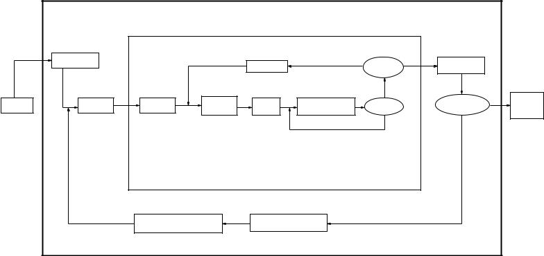
8.3.2.9 Implementation
The algorithm has been implemented in C + + using a template class for volumetric images.2 A synopsis of the algorithm is presented in Fig. 8.3.
8.3.3 Results
8.3.3.1 Intensity Correction
We have evaluated the approach on various MR acquisitions. We present results on real data of the intensity correction, comparing the EM and SEM approaches and comparing the number of Gaussian laws used to model the histogram.
We have tested the approach on various T1-MR images and the algorithm has proved to be robust and reliable. Furthermore, it does not require any spatial alignment between the images to be corrected and can therefore be applied in various contexts: MR time series or MR of different subjects. Figure 8.4 presents cut-planes images of volumetric MR.
Figure 8.5 presents the effect of the correction using a EM algorithm and Fig. 8.6 the correction using a SEM algorithm. For each estimation scheme, we test a mixture of five (left) and seven Gaussian distributions to model the histogram. In each case, a fourth order parametric correction has been estimated.
2 http://www.irisa.fr/vista/Themes/Logiciel/VIsTAL/VIsTAL.html
|
|
|
multiresolution minimization |
|
|
|
|
||
|
|
|
multigrid minimization |
|
|
|
|
||
|
resolution= |
|
|
|
NO |
|
YES |
field = field + |
|
|
coarse_resolution |
|
|
grid = grid − 1 |
Finest grid? |
|
|||
|
|
|
|
|
incremental field |
|
|||
|
|
|
|
|
|
|
|
|
|
|
|
|
|
|
|
YES |
|
|
|
rigid |
filtering |
grid= |
initialize |
initialize |
|
|
|
YES |
Compute |
Gauss Seidel |
convergence? |
|
|
total |
|||||
incremental |
|
Finest resolution? |
|||||||
registration |
subsampling |
coarse_grid |
|
||||||
grid |
minimization |
|
deformation |
||||||
deformation |
|
|
|
||||||
|
|
|
|
|
|||||
|
|
|
|
|
|
|
|
field |
|
|
|
|
|
|
|
|
|
NO |
|
|
|
|
|
|
|
NO |
|
|
|
|
|
|
|
|
|
|
|
|
|
|
|
project field at lowest resolution |
resolution = resolution − 1 |
|
|
|
|
||
|
|
|
|
|
|
|
|
||
Figure 8.3: Overview of the multiresolution and multigrid minimization. The convergence of the multigrid minimization is based on a percentage of cubes for which the parametric incremental field has been updated (percentage of the total number of cubes of the image partition).