

Kluwer - Handbook of Biomedical Image Analysis Vol
.3.pdf350 |
Kybic and Unser |
solution by gradual refinements. We first solve a reduced problem using a small amount of data, then use the solution as an initial guess for the problem at a finer level. This is repeated until the finest (original) level is reached.
Multiresolution on the search space works similarly, adding degrees of freedom to the warping model at each step. We start with a simple model leading to a simple and easy to solve problem. Then gradually add a manageable amount of complexity at each step, until the desired model is reached. The model can be augmented qualitatively, such as going from translation-only to general affine transform, or quantitatively, for example, by decreasing the control node spacing in semi-local models.
Related to multiresolution are multigrid optimization methods, where occasional backward transitions from finer to coarser levels are used besides the coarse-to-fine refinement used in the multiresolution [63].
9.2.5 Other Attributes and Features
The dimensionality refers to the number of dimensions of the images being registered. The warping function normally works in the space of the same dimensionality, transforming one coordinate vector into another.
Interactive algorithms need human supervision and interaction, as opposed to fully autonomous ones. Interactive methods often perform well, taking advantage of the human expert, but are unsuitable for treating high volumes of data. Good compromise might be to use hybrid methods, requiring manual intervention or approval only in difficult cases.
In some cases there is no inherent reference and test image, both can play the same role. Then we would like the registration process to be consistent with respect to this choice [69, 70]. Consistency is one of the ways to enforce invertibility and preservation of the topology of the transformation, other possibilities involve constraining the Jacobian [71] and composition of diffeomorphic mappings [32].
9.2.6 Complementary Surveys
There is a wide choice of sources of information on registration algorithms. The surveys by Brown [5] and a newer one by Zitova´ [72] are rather general. Warfield et al. [73] concentrate on nonlinear registration for brain warping applications.
Elastic Registration for Biomedical Applications |
351 |
Bayesian interpretation of elastic matching are reviewed by Gee [74], also in the context of human neuroanatomy. The last two survey articles we mention deal specifically with medical imaging applications of image registration. An article by Van den Elsen et al. [75] contains very comprehensive and detailed classification of available methods. Finally, Lester and Arridge [76] emphasise the hierarchical concepts of the algorithms.
9.3 Landmark Registration
Landmark registration [1, 19, 20] is a two-step feature-based registration technique. In the first step, a set of landmark pairs is identified (see Fig. 9.2 for an example), either manually, or automatically [20, 77]. We get two sequences of points, x1, . . . , xN , and z1, . . . , zN , such that an object at coordinates xi in the reference image corresponds to the object at coordinates zi in the test image. In the second step, the correspondence function is interpolated between the landmark points [78, 79].
Manual landmark registration has the usual inconveniences of a manual method—poor accuracy and repeatability. On the other hand, it is robust and reliable thanks to the underlying human expert knowledge. For this reason, it is very valuable as a bootstrap method for further automatic refinement. It can also serve as a reference standard when evaluating the performance of other registration methods on real images and under realistic working conditions.
Landmark interpolation merits a study in its own right. Choosing an interpolation method or an interpolation function is difficult because the implications of this choice are not immediately apparent. On the other hand, in the variational formulation we shall present, the user is asked instead to choose a criterion of optimality, which is usually more tangible and often related to the physics (or other specificities) of the problem. The variational formulation of landmark interpolation also allows us to make an interesting link with (fractional) splines [80].
9.3.1 Desirable Properties
The landmark interpolation method should fulfill some basic properties:
352 |
Kybic and Unser |
We agree that landmarks are points in space, as opposed to just coordinate values. Similarly, the correspondence function g is more than a mathematical function: it describes correspondence of real points. It is an object in space, anchored to the landmarks. Consequently, it seems reasonable to require that the interpolated function g be invariant with respect to the choice of the coordinate system. In other words, the correspondence between points in the two images should remain the same, regardless of how we measure the position of these points.
The interpolation problem should always have a solution, if possible a unique one.
Another property worth having is the reproduction of identity [81]. In addition, we might want the reproduction property for other simple transformations, such as shifts or scalings; more generally, affine transformations.
We want the reconstructed correspondence function to be close to the (unknown) true underlying correspondence function. We want the reconstruction error to decrease rapidly with the number of landmarks—the method should have good approximation properties [82]. This way we can adapt the landmark density to ensure that the error is below any a priori given tolerance threshold.
Finally, we want the interpolation procedure to accommodate easily nonexact fits, useful when the landmark positions are only known approximately. In this approximation setting, the reconstructed correspondence function will pass close to the landmarks, making a compromise between the closeness of the fit and the overall smoothness.
9.3.2 Thin-Plate Splines
The use of thin-plate spline technique for landmark interpolation is attributed to Bookstein [1]. Here, we present the method from the variational point of view, as a preparation for the extensions presented in section 9.3.3. Instead of imposing an empirical interpolation formula, the essence of the variational formulation consists of choosing a variational criterion J(g) and then finding among all possible functions passing through the landmarks the one that minimizes
J [83, 84].

Elastic Registration for Biomedical Applications |
353 |
The thin-plate spline method uses the physical model of a thin steel plate [21] with small vertical displacement given by the scalar field g and calculates J as
the strain energy of the plate:
J(g) = |
∂2 g |
|
2 |
|
|
∂2 g |
|
2 |
+ |
∂2 g |
|
2 |
2 g 2 dxdy |
|
|
|
+ 2 |
|
|
|
dxdy = |
(9.1) |
|||||||
∂ x2 |
|
∂ x∂ y |
|
∂ y2 |
where 2 denotes the Laplacian and the right equality is obtained by integration by parts under some conditions on the solution space. The Laplacian energy (9.1) is a member of a more general family of scale and rotation invariant cost functions which satisfy the requirements of section 9.3.1, see also [85, 86]. It is also the simplest criterion that does not penalize affine transforms.
The criterion for the vector form g is taken simply as the sum of the strain energies of the x and y components, J(g) = J(gx) + J(gy). As the constraints g(xi) = zi can be broken into two independent sets for gx and gy, it follows that minimizing J for g is equivalent to minimizing separately for gx and gy. Consequently, we can concentrate on the scalar case here.
9.3.2.1 Interpolation Formula
The correspondence function g(x, y) minimizing (9.1) under interpolation constraints g(xi, yi) = zi is given by
N |
|
g(x, y) = λi (!x − xi!) + a0 x + a1 y + a2 |
|
i=1 |
|
with !x − xi! = %(x − xi)2 + (y − yi)2 = r |
(9.2) |
where (r) is a (r) = r2 log r. It is called radial because it only depends on the Euclidean distance r to its associated data point [87].
The generating function (x) = (x, y) solves the associated Euler-Lagrange (or fundamental) equation
%
x4,y ( x2 + y2) = δ(x, y) (9.3)
where 4 is a two times iterated Laplacian and δ(x, y) is the Dirac distribution. The linear polynomial a0 x + a1 y + a2 in (9.2) is called a kernel term and it appears because it does not contribute to the criterion. The unknown parameters
λi and a0, a1, a2 are determined from the interpolation constraints g(xi, yi) = zi
354 |
|
|
Kybic and Unser |
and from orthogonality conditions |
|
|
|
|
|
|
|
N |
N |
N |
|
λi = 0 |
λi xi = 0 |
λi yi = 0 |
(9.4) |
i=1 |
i=1 |
i=1 |
|
The method we have just briefly described is called thin-plate spline interpolation [1, 85, 86, 88].
9.3.3 Fractional Landmark Interpolation
Although the thin-plate splines have been known to work well, in many applications we might benefit from a wider choice of interpolation functions, while keeping the general spirit and the invariance properties (affine geometrical transformations including scaling) we are interested in. The straightforward way to do it is to consider minimizing different criteria, namely fractional derivatives (in 1D) and fractional Laplacian (in multiple dimensions). In some sense, these are the only reasonable criteria guaranteeing the useful properties described above (see [85, 86] for a more precise statement).
9.3.3.1 The Criterion and The Interpolation Formula
The Laplacian is defined in the space domain by 2 |
2 |
|
|
|
2 |
|||||||||
f = ∂∂ x2f |
+ ∂∂ y2f . In the Fourier |
|||||||||||||
domain we have |
2 |
f = |
2 ˆ |
2 ˆ |
= !ω! |
2 |
ˆ |
|
|
|
|
|
|
|
|
ωx f |
+ ωy f |
|
f , provided that all quantities exist. |
||||||||||
This can be |
extended to |
|
|
|
as |
α |
|
α |
ˆ |
, yielding a general- |
||||
fractional orders |
f |
= !ω! |
|
f |
||||||||||
. |
|
|
|
|
|
|||||||||
|
|
|
|
|
|
|
|
|
(9.1): |
|
|
|
|
|
ized version of the Laplacian based criterion . |
|
|
|
|
|
|||||||||
|
J(g) = |
|
|
|
|
|
!ω!2α |gˆ (ω)|2dω |
|
||||||
|
! α g(x)!2dx |
|
(9.5) |
|||||||||||
To get some intuition, note that in the univariate case we would be measuring the norm of the α-th fractional derivative [89, 90] of g.
There is an interesting relationship between fractional Brownian motion [91] and fractional derivatives, since fractional derivatives whiten the fractional Brownian motion and thus effectively yield an uncorrelated Gaussian white noise. The criterion (9.5) can be therefore interpreted as Bayesian fractal prior (see [88] for details and also Poggio [92] for the non-fractal case), assuming that the underlying true function is close to the fractional Brownian motion model. We then find the solution to our interpolation problem combining this knowledge with the information given by the constraints.

Elastic Registration for Biomedical Applications |
355 |
The Euler-Lagrange equation corresponding to (9.5) is 2α = δ. The solution
for non-special α (read: non-integer) is of the form
N |
λi (!x − xi!) |
with (r) = r2α−2 |
|
||||
g = |
(9.6) |
||||||
i=1 |
|
|
r |
|
|
||
|
|
|
|
|
|
|
|
|
does not appear here due to technical restrictions |
||||||
The polynomial kernel term / |
01 2 |
|
|
||||
of the Fourier domain definition of the criterion (9.5).
9.3.3.2 The Influence of α
The coefficient α translates into the assumed smoothness of the deformation— the higher the α, the smoother the deformation. For practical purposes, we will use 0.5 < α ≈< 5; the interpolation becomes point-wise unstable for smaller
α and does not change much for the larger ones. For α > 1.5 the prior can no longer be interpreted as fractal Brownian motion, although the criterion remains usable.
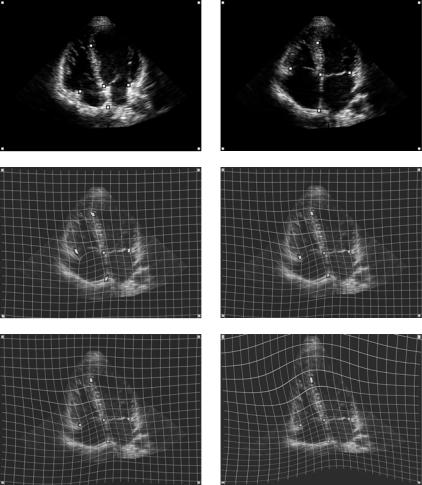
The choice of the order α obviously has an influence on the interpolation results. In Fig. 9.6 we present an example of this effect for the landmark (bivariate) case, (see [86] for additional examples.) We have chosen two images from a four-chamber ultrasound sequence of a heart5 and declared one of them reference and the other a test. We have manually identified six pairs of conforming points in both the images and we have also put additional stable landmarks in the corners of the image. Then we warped the test image onto the reference image varying the parameter α. Note that only non-integer values of α were used, for which the formula (9.6) remains valid; integer values need a special treatment.
How do we choose the best α? As we have seen in the previous section, the statistically optimal α can be determined directly, when the characteristics of the stochastic process generating the deformation are known. However, in practice, this is never the case . Therefore, α must be found experimentally. We observe that small α yields more localized and abrupt changes in the deformation field, while higher α gives rise to smoother and more global changes, as predicted.
5 Acknowledgements: Images and landmark placement are the courtesy of Marıa´ J. Ledesma, Universidad Politecnica´ de Madrid, and Laboratory of Echocardiography, Hospital General Universitario Gregorio Maran˜on,´ Madrid, Spain.
356 |
Kybic and Unser |
Reference |
Test |
alpha=0.5 |
alpha=0.9 |
alpha=1.3 |
alpha=2.5 |
Figure 9.6: The reference (top left) and test (top right) images. The test image warped by landmark warping for α = 0.5 (middle left), α = 0.9 (middle right),
α = 1.3 (bottom left), and α = 2.5 (bottom right). The landmark positions are marked with white squares and were identical in all cases.
When a sufficient number of test images and landmarks are available, a suitable α for a given application can be determined by the leave-one-out technique: One or several landmarks are not taken into consideration when calculating the correspondence function. Their real position is then compared to their position predicted by the interpolation. Finally, the α yielding the smallest average error
Elastic Registration for Biomedical Applications |
357 |
is selected. In the present case, we found the values of α = 1.5 2.5 to be the most suitable.
9.3.4 Summary of Landmark Interpolation
We have presented the landmark registration technique with focus on the second step, the problem of landmark interpolation. This problem can be formulated very concisely in the variational setting. We choose the variational criterion to impose useful properties on the interpolation process, such as rotational, translational, and scale invariance. Most notably, when the criterion is quadratic, the solution is expressed as a linear combination of translated generating (Green) functions. The coefficients of this linear combination are determined from a linear system of equations.
The a priori non-local generating functions can be localized [88] for more efficient and more stable calculation. In some cases this localization leads to B-splines which gives an additional justification for using splines to solve this kind of problems.
9.4Fast Parametric Elastic Image Registration
This section presents a practical example of a fully automatic algorithm for fast elastic multidimensional intensity-based image registration with a parametric B-spline model of the deformation. Its main features are high-order B- spline models of the deformation and of the image, pixel-based similarity criterion, double multiresolution strategy (for both image and the model) and sophisticated iterative multidimensional optimizer. While the algorithm presented here is based on our own work [88, 93–96], it is closely related to a number of similar, independently developed approaches, of which we can only present a very incomplete list. The use of B-spline deformation models was pioneered by Szeliski [40,41] and the different pixel criteria were studied by Studholme [48,97] and Nikou [49]. The hierarchical structure was exploited by Musse [71], Heitz [68] and Thevenaz´ [36], who also employed the Marquardt-Levenberg optimizer.
358 |
Kybic and Unser |
The algorithm can be used for 2D and 3D problems, is reasonably fast, and is capable of accepting expert hints in the form of soft landmark constraints
[1, 19–21].
9.4.1 Problem Formulation
The input images are given as two N-dimensional discrete signals fr (i) and ft (i), where i I ZN , and I is an N-dimensional discrete interval representing the set of all pixel coordinates in the image. We call fr and ft reference and test images, respectively. We suppose that the test image is a geometrically deformed version of the reference image, and vice versa. This is to say that the points with the same coordinate x in the reference image fr (x) and in the warped test image fw (x) = ftc g(x) should correspond. Here, ftc is a continuous version of the test image and g(x) is a deformation (correspondence) function to be identified.
9.4.2 Cost Function
The two images fr , fw will not be identical because of noise and also because the assumption that there is a geometrical mapping between the two images is not necessarily correct. Therefore, we define the solution to our registration problem as the result of the minimization g = arg ming G E(g), where G is the space of all admissible deformation functions g. We have chosen the SSD (sum of squared differences) criterion
|
1 |
|
|
1 |
|
|
||
E = |
!I! i |
I |
ei2 = |
!I! i |
I ( fw (i) − fr (i))2 |
|
||
|
|
|
|
|
|
|
|
|
|
|
|
|
|
1 |
|
|
|
|
|
|
|
= |
!I! i |
I ( ftc(g(i)) − fr (i))2 |
(9.7) |
|
|
|
|
|
|
|
|
|
|
because it is fast to evaluate and yields a smooth criterion surface which lends itself well to optimization. Minimization of (9.7) yields the optimal solution g in the ML (maximum likelihood) sense under the assumption that fr is a deformed (warped) version of ft with i.i.d. (independent and identically distributed) Gaussian noise added to each pixel. The SSD criterion proved to be robust enough, especially if preprocessing was used to equalize the image values—we mostly applied high-pass filtering and histogram normalization [98]. In principle, there

Elastic Registration for Biomedical Applications |
359 |
is no difficulty in extending this method for more sophisticated pixel-based similarity measures, such as information-based measures [99], especially mutual information [45], or weighted p norms. Only the evaluation of the criterion and its derivatives (gradient) needs to be changed.
9.4.3 B-Splines and Image Interpolation
We have chosen to interpolate the image using uniform B-splines:
|
(9.8) |
ftc(x) = i Ib ZN biβn(x − i) |
where βn(x) is a tensor product of B-splines βn(x) of degree n, i.e., βn (x) =
3
N |
βn(xk), with x = (x1, . . . , xN ). Mirror boundary conditions were used, to |
k=1 |
ensure continuity.
Let us recall some basic facts about B-splines. Uniform symmetric B- splines [100] of degree n are piecewise polynomials of degree n. The polynomial pieces are delimited by uniformly placed knots. B-splines of degree n have continuous derivatives up to order n − 1 everywhere. Their integer shifts form a basis. The first (degree zero) symmetric B-spline is defined as β0(x) = 1 for x (− 12 , 12 ) and 0 otherwise. Higher order B-splines are defined recursively as βn+1 = βn β0 and their support is (− n+2 1 , + n+2 1 ).
Using B-splines as interpolation functions has many advantages: B-splines have good approximation properties—for example, the error of a cubic B-spline (β3) approximation decreases asymptotically as h4 (measured by any L p or l p norm, p {1, 2, . . . , ∞}). B-splines perform well in comparison with other bases [11, 101]. B-splines are fast—they have a short support (length 4 for β3), are symmetric, piecewise cubic, and separable in multiple dimensions. They are simple to compute and scalable—the transition from a coarse spline space with step size (knot distance) h q to a finer space with step size h is exact for integer q.
9.4.4 Deformation Model Structure
So far, we have considered the deformation function g to be an arbitrary admissible function RN → RN . We will restrict it now to a family of functions described