Kluwer - Handbook of Biomedical Image Analysis Vol

G., Pennec, X., Noz, M.E., Maguire, G.Q., Jr., Pollack, M., Pelizzari, C.A., Robb, R.A., Hanson, D. and Woods, R.P., Comparison and evaluation of retrospective intermodality brain image registration techniques, Journal of Computer Assisted Tomography, Vol. 21, pp. 554–566, 1997.

[9]Fitzpatrick, J.M., Hill, D.L.G., Shyr, Y., West, J., Studholme, C. and Maurer, C.R., Jr., Visual assessment of the accuracy of retrospective registration of MR and CT images of the brain, IEEE Transactions on Medical Imaging, Vol. 17, No. 4, pp. 571–585, Aug. 1998.

[10]West, J., Fitzpatrick, J.M., Wang, M.Y., Dawant, B.M., Maurer, C.R., Jr., Kessler, R.M. and Maciunas, R.J., Retrospective intermodality registration techniques for images of the head: Surface-based versus volumebased, IEEE Transactions on Medical Imaging, Vol. 18, No. 2, pp. 144– 150, Feb. 1999.

[11]Studholme, C., Hill, D.L.G. and Hawkes, D.J., Automatic threedimensional registration of magnetic resonance and positron emission tomography brain images by multiresolution optimization of voxel similarity measures, Medical Physics, Vol. 24, No. 1, pp. 25–35, Jan. 1997.

[12]Penney, G.P., Weese, J., Little, J.A., Desmedt, P., Hill, D.L.G. and Hawkes, D.J., A comparison of similarity measures for use in 2D-3D medical image registration, IEEE Transactions on Medical Imaging, Vol. 17, No. 4, pp. 586–595, 1998.

[13]Holden, M., Hill, D.L.G., Denton, E.R.E., Jarosz, L.M., Cox, T.C.S., Rohlfing, T., Goodey, J. and Hawkes, D.J., Voxel similarity measures for 3D serial MR brain image registration, IEEE Transactions on Medical Imaging, Vol. 19, No. 2, pp. 94–102, 2000.

[14]Wells, W.M., III, Viola, P.A., Atsumi, H., Nakajima, S. and Kikinis, R., Multimodal volume registration by maximization of mutual information, Medical Image Analysis, Vol. 1, No. 1, pp. 35–51, 1996.

[15]Maes, F., Collignon, A., Vandermeulen, D., Marchal, G. and Suetens, P., Multimodality image registration by maximization of mutual information, IEEE Transactions on Medical Imaging, Vol. 16, No. 2, pp. 187–198, April 1997.

[16]Tsao, J., Interpolation artifacts in multimodality image registration based on maximization of mutual information, IEEE Transactions on Medical Imaging, Vol. 22, No. 7, pp. 854–864, July 2003.

[17]Pluim, J.P., Maintz, J.B.A. and Viergever, M.A., Mutual informationbased registration of medical images: A survey, IEEE Transactions on Medical Imaging, Vol. 22, No. 8, pp. 986–1004, August 2003.

[18]Zhu, Y.M., Volume image registration by cross-entropy optimization, IEEE Transactions on Medical Imaging, Vol. 21, No. 2, pp. 174–180, Feb. 2002.

[19]Shore J.E. and Johnson, R.W., Axiomatic derivation of the principle of maximum entropy and the principle of minimum crossentropy, IEEE Transactions on Information Theory, Vol. 26, No. 1, Jan. 1980.

[20]Johnson R.W. and Shore, J.E., Comments on and correction to Axiomatic derivation of the principle of maximum entropy and the principle of minimum cross-entropy, IEEE Transactions on Information Theory, Vol. 29, No. 6, Nov. 1983.

[21]Shore J.E. and Johnson, R.W., Properties of cross-entropy minimization, IEEE Transactions on Information Theory, Vol. 27, No. 4, July 1981.

[22]Shore, J.E., Minimum cross-entropy spectral analysis, IEEE Transactions on Acoustics, Speech, and Signal Processing, Vol. 29, No. 2, pp. 230–237, 1981.

[23]Zhuang, T.G., Zhu, Y.M. and Zhang, X.L., Minimum cross-entropy algorithm (MCEA) for image reconstruction from incomplete projection, SPIE, Vol. 1606, pp. 697–704, 1991.

[24]Yee, E., Reconstruction of the antibody-affinity distribution from experimental binding data by a minimum cross-entropy procedure, Journal of Theoritical Biology, Vol. 153, No. 2, pp. 205–227, Nov. 1991.

[25]Alwan, L.C., Ebrahimi, N. and Soofi, E.S., Information theoretic framework for process control, European Journal of Operational Research, Vol. 111, No. 3, pp. 526–542, Dec. 1998.

[26]Das, N.C., Mazumder, S.K. and De, K., Constrained non-linear programming: A minimum cross-entropy algorithm, Engineering Optimization, Vol. 31, No. 4, pp. 479–487, 1999.

[27]Antolin, J., Cuchi, J.C., and Angulo, J.C., Minimum cross-entropy estimation of electron pair densities from scattering intensities, Physics Letters A, Vol. 26, pp. 247–252, Sept. 1999.

[28]Zhu, Y.M. and Wang, Z.Z., Minimum reversed cross-entropy spectral analysis, Chinese Signal Processing, Vol. 8, No. 2, pp. 86–90, 1992.

[29]Yang, Z.G. and He, Z.Y., A novel method for high resolution spectral analysis—minimum symmetric divergence spectral analysis, Acta Electronica Sinica, Vol. 17, No. 2, 1989.

[30]Liou, C.Y. and Lin, S.L., The other variant Boltzmann machine, International Joint Conference Neural Networks, Vol. 1, pp. 449–454, 1989.

[31]Kotz, D., Nuclear medicine in the 21st century: Integration with other specialties, Journal of Nuclear Medicine, Vol. 40, No. 7, pp. 13N–25N, July 1999.

[32]Tarantola, G., Zito, F. and Gerundini, P., PET instrumentation and reconstruction algorithms in whole-body applications, Journal of Nuclear Medicine, Vol. 44, No. 5, pp. 756–769, May 2003.

[33]Boes, J.L. and Meyer, C.R., Multivariate mutual information for registration, in Medical Image Computing and Computer-Assisted Intervention—MICCAI’99, Taylor C. and Colchester, A., eds., pp. 606– 612, Springer-Verlag, 1999.

[34]Leventon, M.E. and Grimson, W.E., Multimodal volume registration using joint intensity distribution, Lecture Notes on Computer Sciences, Vol. 1496, pp. 1057–1066, Oct. 1998.

[35]Andersson, J.L.R., Sundin, A. and Valind, S., A Method for coregistration of PET and MR brain images, Journal of Nuclear Medicine, Vol. 36, pp. 1307–1315, 1995.

[36]Zhu, Y.M. and Cochoff, S.M., Likelihood maximization approach to image registration, IEEE Transactions on Image Processing, Vol. 11, No. 12, pp. 1417–1426, Dec. 2002.

[37]Foley, J.D., Van Dam, A., Feiner, S.K. and Hughes, J.F., Computer Graphics: Principles and Practice, 2nd edn., Addison-Wesley, Reading, MA, 1996.

[38]Zhu, Y.M. and Cochoff, S.M., Influence of implementation parameters on mutual information maximization image registration of MR/SPECT brain images, Journal of Nuclear Medicine, Vol. 43, No. 2, pp. 160–166, Feb. 2002.

[39]Press, W.H., Teukolsky, S.A., Vetterling, W.T. and Flannery, B.P., Numerical Recipes in C: the Art of Scientific Computing, Cambridge University Press, Cambridge, 1999.

[40]Ritter, N., Owens, R., Cooper, J., Eikelboom, R.H. and Van Saarloos, P.P., Registration of stereo and temporal images of the retina, IEEE Transactions on Medical Imaging, Vol. 18, No. 5, pp. 404–418, May 1999.

[41]Fitzpatrick, J.M., Hill, D.L.G. and Maurer, C.R., Image Registration In: Handbook of Medical Imaging: Vol. 2, Medical Image Processing and Analysis, Sonka, M. and Fitzpatrick, J.M., eds, SPIE Press, Bellingham, 2000.

[42]Maes, F., Vandermeulen, D. and Suetens, P. Comparative evaluation of multiresolution optimization strategies for multimodality image registration by maximization of mutual information, Medical Image Analysis, Vol. 3, No. 4, pp. 373–386, 1999.

[43]Pelizzari, C.A., Chen, G.T.Y., Spelbring, D.R., Weichselbaum, R.R. and Chen, C.T., Accurate three-dimensional registration of CT, PET, and/or MR images of the brain, Journal of Computer Assisted Tomography, Vol. 13, No. 1, pp. 20–26, 1989.

[44]Costa, W.L.S., Haynor, D.R., Haralick, R.M., Lewellen, T.K. and Graham, M.M., A maximum-likelihood approach to pet emission/attenuation image registration, IEEE Nuclear Science Symposium and Medical Imaging Conference, pp. 1139–1143, 1993.

[45]Liebig, J.R., Jones, S.M. and Wang, X., Coregistration of multimodality data in a medical imaging system, US Patent 5,672,877. 1997.

[46]Dey, D., Slomka, P.J., Hahn, L.J. and Kloiber, R., Automatic threedimensional multimodality registration using radionuclide transmission CT attenuation maps: A phantom study, Journal of Nuclear Medicine, Vol. 40, pp. 448–455, 1999.

[47]Kiebel, S.J., Ashburner, J., Poline, J.B. and Friston, K.J., MRI and PET coregistration—A cross validation of statistical parametric mapping and automatic image registration, Neuroimage, Vol. 5, pp. 271–279, 1997.

magnetic resonance (MR) imaging, or by a combination of images of the same object acquired from different imaging modalities in general.

There are, however, many applications where there is no well-defined relationship between a voxel’s value(s) and the label that should be assigned to it. This observation is fairly obvious when we are seeking to label anatomical structures rather than tissue types. It is clear, for example, different structures that are composed of the same tissue (e.g., different bones) cannot be distinguished from one another by looking at their intensity values in an image. What distinguishes these structures instead is their location and their spatial relationship to other structures. In such cases, spatial information (e.g., neighborhood relationships) therefore needs to be taken into consideration and included in the segmentation process.

Level set methods [37, 66, 75, 86] simultaneously segment all voxels that belong to a given anatomical structure. Starting from a seed location, a discrete set of labeled voxels is evolved according to image information (e.g., image gradient) and internal constraints (e.g., smoothness of the resulting segmented surface). Snakes or active contours [85] use an analytical description of the segmented geometry rather than a discrete set of voxels. Again, the geometry evolves according to the image information and inherent constraints.

In addition to geometrical constraints, one can take into account neighborhood relationships between several different structures [74, 84]. A complete description of such relationships is an atlas. In general, an atlas incorporates the locations and shapes of anatomical structures, and the spatial relationships between them. An atlas can, for example, be generated by manually segmenting a selected image. It can also be obtained by integrating information from multiple segmented images, for example, from different individuals. We shall discuss this situation in more detail in section 11.4.3.

Given an atlas, an image can be segmented by mapping its coordinate space to that of the atlas in an anatomically correct way, a process commonly referred to as registration. Labeling an image by mapping it to an atlas is consequently known as atlas-based segmentation, or registration-based segmentation. The idea is that, given an accurate coordinate mapping from the image to the atlas, the label for each image voxel can be determined by looking up the structure at the corresponding location in the atlas under that mapping. Obviously, computing the coordinate mapping between the image and the atlas is the critical step in any such method. This step will be discussed in some detail in section 11.3.

A variety of atlas-based segmentation methods have been described in the literature [3, 11, 12, 15, 16, 21, 23, 24, 38, 41]. The characterizing difference between most of these methods is the registration algorithm that is used to map the image coordinates onto those of the atlas. One important property, however, is shared among all registration methods applied for segmentation: as there are typically substantial shape differences between different individuals, and therefore between an individual and an atlas, the registration must yield a non-rigid transformation capable of describing those inter-subject deformations.

In this chapter we take a closer look at an often neglected aspect of atlasbased segmentation, the selection of the atlas. We give an overview of the different strategies for atlas selection, and demonstrate the influence of the selection method on the accuracy of the final segmentation.

11.2From Subject to Atlas: Image Acquisition and Processing

We illustrate the methods and principles discussed in this chapter by segmenting confocal microscopy images from 20 brains of adult, honeybee workers. Confocal laser scanning microscopy is a type of fluorescence microscopy, where a focused laser beam deflected by a set of xy-scanning mirrors excites the fluorescently stained specimen (i.e., the dissected brain). The emitted fluorescence is then recorded by inserting a so-called “confocal pinhole” into the microscope’s optical path. This pinhole ensures that only light from the focal plane reaches the detector, thus enabling the formation of an image that can be considered an optical section through the specimen. By moving the position of the specimen along the optical axis of the microscope a three-dimensional (3D) image is generated [8, 69, 88]

The staining of the bee brains depicted in this chapter followed an adapted immunohistological protocol. Dissected and fixated brains were incubated with two primary antibodies (nc46, SYNORF1) that detect synapse proteins [28, 46]. Because cell bodies in insects reside separately from fibers and tracts, this staining ensures response from those regions in the tissue that exhibit high synaptic densities, i.e., neuropil, while somata regions remain mostly unstained. A Cy3-conjugated secondary antibody sensitive to the constant part of the primary

antibody was subsequently used to render labeled regions fluorescent. After dehydration and clearing, the specimens were mounted in double-sided custom slides.

The brains were imaged with a confocal laser scanning microscope (Leica TCS 4D). The chromophor was excited with an ArKr laser, and the fluorescence was detected using a longpass filter. The intensity of the fluorescence was quantized with a resolution of 8 bits. Due to the size of the dissected and embedded brain (about 2.5 × 1.6 mm laterally and about 0.8 mm axially), it cannot be imaged in a single scan. Therefore we used multiple image-stack acquisition (3DMISA) [88]. The entire brain was scanned in 2 × 3 partially overlapping single scans, each using 512 × 512 pixels laterally and between 80 and 120 sections axially. The stacks were combined into a single 3D image using custom software or a script running in Amira (see next paragraph). Because of the refractive index mismatch between the media in the optical path, images exhibit a shortening of distances in axial direction that was accounted for by a linear scaling factor of

1.6[7].

Post-acquisition image processing was done with the Amira 3D scientific

visualization and data analysis package (ZIB, Berlin, Germany; Indeed – Visual Concepts GmbH, Berlin, Germany; TGS Inc., San Diego, CA). Image stacks were resampled laterally to half of the original dimensions in order to increase display speeds and allow interactive handling of the data. The final image volume contained 84–114 slices (sections) with thickness 8 m. Each slice had 610–749 pixels in x direction and 379–496 pixels in y direction with pixel size 3.8 m. In most cases no further image processing was necessary. In a few cases unsharp masking filters were applied in order to enhance contours.

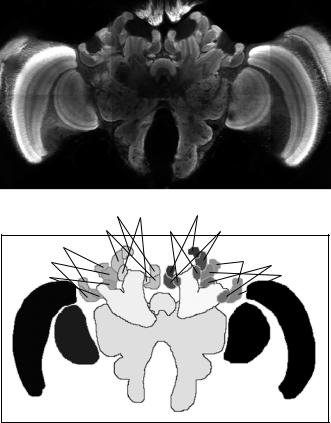
Subsequently, for each brain an atlas of the neuropil areas of interest was generated by tracing them manually on each slice. We distinguished 22 major compartments, 20 of which are bilaterally symmetric on either brain hemisphere [39]. The paired structures we labeled were medulla, lobula, antennal lobe, ventral mushroom body consisting of peduncle, α- and β-lobe, and medial and lateral lip, collar and basal ring neuropil. The unpaired structures we identified were the central body with its upper and lower division and the protocerebral lobes including the subesophageal ganglion. Examples of confocal microscopy and label images are shown in Fig. 11.1. Three-dimensional surface renderings of the segmented bee brain are shown in Fig. 11.2. The labeled structures and the abbreviations used for them in this chapter are listed in Table 11.1.