Kluwer - Handbook of Biomedical Image Analysis Vol
.3.pdf

462 Rohlfing et al.
to effectively compare different segmentation methods, we need to quantify the
segmentation accuracy. One possible measure of segmentation quality is the similarity index (SI) [87]. For a structure s, the SI is computed from the set
V (s) |
of voxels in s according to the automatic segmentation and the set V (s) |
|||||||||||||
auto |
|
|
|
|
|
|
|
|
|
|
|
|
|
manual |
of voxels in s according to the (gold standard) manual segmentation: |
|
|||||||||||||
|
|
= |
|
V |
V (s) |
|
|
|
V |
(s) |
|
|
|
|
|
|
|
2 |
|
|
|
|
V |
|
|
|
|||
|
|
|
|
|
|
manual |
|
|
auto |
|
|
|
||
|
SI(s) |
|
|
|
(s) |
+ |
|
|
(s) |
|
|
(11.8) |
||
|
|
|
|
|
∩ |
|
. |
|||||||
|
|
|
|
manual |
|
|
|
|
|
|
||||
|
|
|
|
|
|
|
|
|
|
|
|
|||
|
|
|
|
|
|
|
|
auto |
|
|||||
For perfect mutual overlap of both segmentations, manual and automatic, the SI has a value of 1. Lesser overlap results in smaller values of SI. No overlap between the segmentations results in an SI value of 0. A major advantage of the SI measure is that it is sensitive to both over-segmentation and under-segmentation, that is, it recognizes both false positives and false negatives among the voxels of a given structure.
11.5.2 Bias from Structure Volume
In order to understand the SI values computed later in this chapter and to compare them with other published values, we investigated the dependence of SI values on object size. We performed a numerical simulation in which discretely sampled spheres of various radii were dilated by one or two voxels and the SI values between the original and dilated spheres were computed. The resulting SI values are plotted versus object radius in Fig. 11.12. It is also easy to derive a closed-form expression for the continuous case. The SI between two concentric spheres, one with radius R and the other dilated by d, i.e., with a radius of R + d, is
2(R/d)3
SI = . (11.9) 2(R/d)3 + 3(R/d)2 + 3(R/d) + 1
The SI values for the discrete and continuous cases are almost identical (Fig. 11.12). The SI value between a sphere and a concentric dilated sphere approximates the SI value for a segmentation error consisting of a uniform thickness misclassification on the perimeter of a spherical object. Inspection of Fig. 11.12 and Eq. (11.9) shows that SI depends strongly on object size and is smaller for smaller objects. A one voxel thick misclassification on the perimeter of a spherical object with a radius of 50 voxels has an SI value of 0.97, but for a radius of 10 voxels the SI value is only 0.86. Thus it is not surprising that Dawant

464 |
Rohlfing et al. |
|
|
1000 |
|
|
|
|
|
|
|
|
|
|
|
|
|
|
|
|
|
|
|
|
1.00 |
|
Average Volume Over 20 Bee |
Brains (1000s of voxels) |
900 |
|
|
|
|
|
|
|
|
|
|
|
|
|
|
|
|
|
|
|
|
0.90 |
|
800 |
|
|
|
|
|
|
|
|
|
|
|
|
|
|
|
|
|
|
|
|
0.80 |
Similarity Index (MUL) |
||
700 |
|
|
|
|
|
|
|
|
|
|
|
|
|
|
|
|
|
|
|
|
0.70 |
|||
600 |
|
|
|
|
|
|
|
|
|
|
|
|
|
|
|
|
|
|
|
|
0.60 |
|||
500 |
|
|
|
|
|
|
|
|
|
|
|
|
|
|
|
|
|
|
|
|
0.50 |
|||
400 |
|
|
|
|
|
|
|
|
|
|
|
|
|
|
|
|
|
|
|
|
0.40 |
|||
300 |
|
|
|
|
|
|
|
|
|
|
|
|
|
|
|
|
|
|
|
|
0.30 |
|||
200 |
|
|
|
|
|
|
|
|
|
|
|
|
|
|
|
|
|
|
|
|
0.20 |
|||
100 |
|
|
|
|
|
|
|
|
|
|
|
|
|
|
|
|
|
|
|
|
0.10 |
|||
0 |
|
|
|
|
|
|
|
|
|
|
|
|
|
|
|
|
|
|
|
|
0.00 |
|||
|
|
|
|
|
|
|
|
|
|
|
|
|
|
|
|
|
|
|
|
|
|
|
||
|
|
vPKl |
vPKr |
Cb |
LPL-USG |
rmbR |
rmLip |
rmColl |
rlLip |
rlColl |
rlbR |
llLip |
llColl |
llbR |
lmbR |
lmColl |
lmLip |
rLobula |
rMedulla |
lMedulla |
lLobula |
lal |
ral |
|
Anatomical Structure
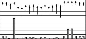
Figure 11.13: Volumes of anatomical structures and corresponding segmentation accuracies. The gray bars show the volumes (in numbers of voxels) of the 22 anatomical structures, averaged over the 20 bee brains. The black vertical lines show the range of SI values achieved by the automatic segmentation (MUL paradigm) over all segmented raw images. The diamond shows the median over all segmented raw images.
A surface voxel is easily defined as one that has a neighbor with a label different from its own. When the entire surface of a structure is misclassified, this can be seen as an erosion of the structure by one voxel. The SI value computed between the original structure and the eroded structure represents the SI resulting from a segmentation that misclassifies exactly all surface voxels. From the structure’s SVR ρ and its total volume V , this SI can be computed as
SI |
|
|
2V (1 − ρ) |
= |
1 − ρ |
. |
(11.11) |
|||||
= V |
|
|
||||||||||
|
+ |
(1 |
− |
ρ)V |
1 |
− |
ρ/2 |
|
||||
|
|
|
|
|
||||||||
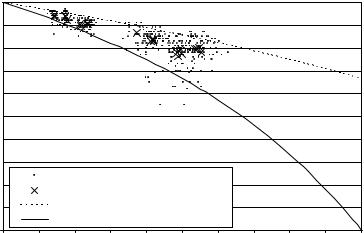
Similarly, we can estimate the SI resulting from a misclassification of half of all surface voxels. Figure 11.14 shows the SVR values computed for all structures in all brains in our 20 bee brains, plotted versus the SI values of the automatic segmentations. The figure also shows two curves that represent the theoretical misclassification of all and half of all surface voxels, respectively.
For a typical segmentation result of a single structure, a detailed comparison of manual and automatic segmentation is shown in Fig. 11.15. The structure shown here, a right ventral mushroom body, is typical in that its volume and
Quo Vadis, Atlas-Based Segmentation? |
465 |
|
1 |
|
|
|
|
|
|
|
|
|
|
|
0.9 |
|
|
|
|
|
|
|
|
|
|
|
0.8 |
|
|
|
|
|
|
|
|
|
|
Index |
0.7 |
|
|
|
|
|
|
|
|
|
|
0.6 |
|
|
|
|
|
|
|
|
|
|
|
|
|
|
|
|
|
|
|
|
|
|
|
Similarity |
0.5 |
|
|
|
|
|
|
|
|
|
|
0.4 |
|
|
|
|
|
|
|
|
|
|
|
0.3 |
|
|
|
|
|
|
|
|
|
|
|
|
|
|
|
|
|
|
|
|
|
|
|
|
0.2 |
|
Individuals |
|
|
|
|
|
|
|
|
|
|
Mean for one structure over all individuals |
|
|
|
|
|||||
|
|
|
|
|
|
|
|||||
|
0.1 |
|
Erosion by 1/2 voxel |
|
|
|
|
|
|
|
|
|
|
|
|
|
|
|
|
|
|
|
|
|
|
|
Erosion by one voxel |
|
|
|
|
|
|
|
|
|
0 |
|
|
|
|
|
|
|
|
|
|
|
0 |
0.1 |
0.2 |
0.3 |
0.4 |
0.5 |
0.6 |
0.7 |
0.8 |
0.9 |
1 |
Surface-to-Volume Ratio
Figure 11.14: Similarity index vs. surface-to-volume ratio. Each dot represents one structure in one brain (418 structures in total). The average over all individuals for one structure is marked by a ×. The solid and dashed lines show the theoretical relationship between SVR and SI for misclassification of all and half of all surface voxel, respectively.
its surface-to-volume ratio are close to the respective means over all structures (volume 141k pixels vs. mean 142k pixels; SVR 0.24 vs. mean 0.36). The segmentation accuracy for the segmentation shown was SI = 0.86, which is the median SI value over all structures and all brains.
11.5.4 Comparison of Atlas Selection Strategies
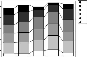
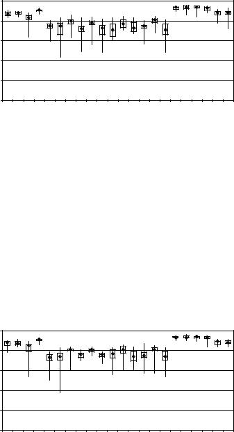
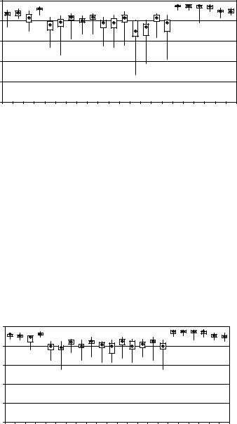
The results achieved using the different atlas selection strategies outlined above are visualized in Figs. 11.16–11.19. Each graph shows a plot of the distribution of the SI segmentation accuracies over 19 segmentations, separated by anatomical structure. There were 19 segmentations per strategy as one out of the 20 available bee brain images served as the fixed individual atlas for the IND strategy. Therefore, this brain was not available as the raw image for the remaining strategies, in order to avoid bias of the evaluation.
A comparison of all four strategies is shown in Fig. 11.20. It is easy to see from the latter figure that the widely used IND strategy produced the least accurate
466 |
Rohlfing et al. |
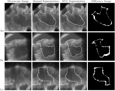
Figure 11.15: A typical segmented structure: right ventral mushroom body (SI = 0.86). Columns from left to right: microscopy image, contour from manual segmentation, contour from automatic segmentation (MUL paradigm), and difference image between manual and automatic segmentation. The white pixels in the difference image show where manual and automatic segmentation disagree.
Rows from top to bottom: axial, sagittal, and coronal slices through the right ventral mushroom body.
results of all strategies. Only slightly better results were achieved by selecting a different individual atlas for each raw image, based on the NMI after non-rigid registration criterion discussed in section 11.4.2. The AVG strategy, segmentation using an average shape atlas, outperformed both the IND and SIM strategies, but was itself clearly outperformed by the MUL strategy. Our results therefore show that the multiclassifier approach to atlas-based segmentation produced substantially more accurate segmentations than the other three strategies. This finding is, in fact, statistically significant when performing a t-test on the SI values for all structures over all segmentations, which confirms the experience of
468 |
Rohlfing et al. |
|
1.00 |
|
|
|
|
|
|
|
|
|
|
|
|
|
|
|
|
|
|
|
|
|
Index |
0.80 |
|
|
|
|
|
|
|
|
|
|
|
|
|
|
|
|
|
|
|
|
|
0.60 |
|
|
|
|
|
|
|
|
|
|
|
|
|
|
|
|
|
|
|
|
|
|
Similarity |
0.40 |
|
|
|
|
|
|
|
|
|
|
|
|
|
|
|
|
|
|
|
|
|
0.20 |
|
|
|
|
|
|
|
|
|
|
|
|
|
|
|
|
|
|
|
|
|
|
|
|
|
|
|
|
|
|
|
|
|
|
|
|
|
|
|
|
|
|
|
|
|
|
0.00 |
|
|
|
|
|
|
|
|
|
|
|
|
|
|
|
|
|
|
|
|
|
|
vPKl |
vPKr |
Cb |
LPL-USG |
rmbR |
rmLip |
rmColl |
rlLip |
rlColl |
rlbR |
llLip |
llColl |
llbR |
lmbR |
lmColl |
lmLip |
rLobula |
rMedulla |
lMedulla |
lLobula |
lal |
ral |
Anatomical Structure
Figure 11.18: SI by label for segmentation using a single average shape atlas (AVG atlas selection strategy) [reproduced from [53]].
11.6More on Segmentation with Multiple Atlases
We saw in the previous section that a multiclassifier approach to atlas-based segmentation outperforms atlas-based segmentation with a single atlas, be it an individual atlas, an average atlas, or even the best out of a database of atlases. Compared to that, the insight underlying the SIM (“most similar”) atlas selection
|
1.00 |
|
|
|
|
|
|
|
|
|
|
|
|
|
|
|
|
|
|
|
|
|
|
0.80 |
|
|
|
|
|
|
|
|
|
|
|
|
|
|
|
|
|
|
|
|
|
Index |
0.60 |
|
|
|
|
|
|
|
|
|
|
|
|
|
|
|
|
|
|
|
|
|
|
|
|
|
|
|
|
|
|
|
|
|
|
|
|
|
|
|
|
|
|
|
|
Similarity |
0.40 |
|
|
|
|
|
|
|
|
|
|
|
|
|
|
|
|
|
|
|
|
|
0.20 |
|
|
|
|
|
|
|
|
|
|
|
|
|
|
|
|
|
|
|
|
|
|
|
0.00 |
|
Cb |
|
|
|
|
|
|
|
|
|
|
|
|
|
|
|
|
|
|
|
|
vPKl |
vPKr |
LPL-USG |
rmbR |
rmLip |
rmColl |
rlLip |
rlColl |
rlbR |
llLip |
llColl |
llbR |
lmbR |
lmColl |
lmLip |
rLobula |
rMedulla |
lMedulla |
lLobula |
lal |
ral |
Anatomical Structure
Figure 11.19: SI by label for segmentation by combining multiple independent
atlas-based segmentations (MUL atlas selection strategy) [reproduced from
[53]].