Kluwer - Handbook of Biomedical Image Analysis Vol

Figure 11.6: Depiction of the atlas selection strategies discussed in this chapter. The strategies are also categorized in Table 11.2. Note that the basic atlas-based segmentation with a single atlas (IND, gray box) occurs in different stages in the other three strategies, in the MUL case replicated for each atlas.

A schematic graphical comparison of the four methods is given in Fig. 11.6, and a textual summary of the categorization can be found in Table 11.2.

For each strategy, the resulting segmentation accuracy was evaluated. Automatic segmentations were compared to a manual gold standard segmentation. A detailed description of the methods used for validation and accuracy evaluation,

Table 11.2: Categorization of atlas selection strategies by number, type, and assignment of atlases. See Sections 11.4.1 through 11.4.4 for details and Fig. 11.6 for a schematic overview of the different methods

together with the results for the four atlas selection strategies, are presented in Section 11.5.

11.4.1Segmentation with a Fixed, Single Individual Atlas

The most straight forward strategy for selection of an atlas is to use one individual segmented image. The selection can be random, or based on heuristic criteria such as image quality, lack of artifacts, or normality of the imaged subject. This strategy is by far the most commonly used method for creating and using an atlas [25]. It requires only one atlas, which greatly reduces the preparation effort as compared to the more complex methods described below.

Out of the 20 bee brains in our population, we picked the one that was judged to have the best image quality and least artifacts. We then used this atlas brain to segment the remaining 19 brain images. Each of the 19 raw images was registered non-rigidly to the microscopy image of the atlas, and labeled using the accordingly transformed atlas label image.

11.4.2 Segmentation with the Best Atlas for an Image

Suppose that instead of a single atlas, we have several atlases that originate from several different subjects. For each image that we are segmenting, there is one atlas that will produce the best segmentation accuracy among all available atlases. It is obviously desirable to use this optimum atlas, which is most likely a different atlas for each image.

Criterion for Most Similar Atlas

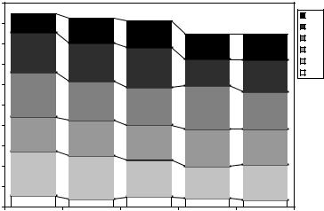
Figure 11.7: Percentages of structures segmented with accuracy better than given SI thresholds using different “most similar” atlas selection criteria. Each column represents one criterion (see text for details). The stacked bars from bottom to top show the percentages of structures that were segmented with SI better than 0.95 through 0.70. For comparison, the left-most column shows the results when the atlas with the best a posteriori SI segmentation result is used for each raw image. This is the upper bound for the accuracy achievable with any criterion for selection of the best single individual atlas.

the atlas candidates was chosen using each of the criteria above. The accuracy of a segmentation was computed as the SI between the segmentation and the manual gold standard.

Figure 11.7 shows a graph of the percentages of structures segmented with varying levels of accuracy. For comparison, this graph includes results achieved when using the best atlas according to the a posteriori SI values for each raw image (left-most column, Best SI). In other words, this column shows the best possible result that can be achieved using only a single individual atlas, where the selection of this atlas is governed by the knowledge of the resulting segmentation accuracy (SI value). Obviously, this is not a strategy that is available in practice. However, it provides the upper bound for the segmentation accuracy that can be achieved using any criterion for selection of the best atlas for a given raw image.

Among the four criteria that do not depend on the a posteriori accuracy evaluation and thus a gold standard, the NMI image similarity after non-rigid registration performed slightly better than the other three. It was therefore selected as the criterion used for the SIM atlas selection strategy in the comparison to the other three strategies later in this chapter (section 11.5.4).

11.4.3 Segmentation with an Average Shape Atlas

As we stated in the previous chapter, atlas-based segmentation is an easier task if the atlas is similar to the image that is to be segmented. Smaller magnitudes of the deformation between image and atlas that the non-rigid registration algorithm has to determine typically result in a higher accuracy of the matching. If the atlas is itself derived from an individual subject, then the risk is high that this individual is an outlier in the population. In such a case segmenting other subjects using the atlas becomes a more difficult problem. A better atlas would be one that is as similar to as many individuals as possible. Such an atlas can be generated by creating an average over many individuals.

For the human brain, such an average atlas is available from the Montreal Neurological Institute (MNI) as the BrainWeb phantom [5, 13]. Note, however, that the BrainWeb phantom is an atlas of brain tissue types, so as we discussed in section 11.1, it is not as useful for atlas-based segmentation as an atlas of brain structures. For the human heart, an average atlas derived from cardiac MR images [45] has been used for atlas-based segmentation [35]. Similarly, an average atlas of the lung has been derived from CT images [33].

For demonstration in this chapter, we have therefore generated an average shape atlas of the structures of the bee brain using a technique outlined below [51].

11.4.3.1 Iterative Shape Averaging

One way of obtaining an average shape atlas from a population of subjects is to generate an active shape model (ASM). In short, an ASM provides a statistical description of a population of subjects by means of an average shape and the principal modes of variation [14, 34]. Generating an ASM typically requires the identification of corresponding landmarks on all individuals, a tedious and errorprone process despite recent success in automating this step using non-rigid

wise choice of the initial transformation is therefore beneficial for the robustness of the registration method.

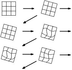
During the iterative averaging process, there are only minor changes in the overall shape of the average brain from one iteration to the next. Consequently, for all images n and all iterations i, the transformation T(ni+1) differs from the preceding T(ni) only by a small additional deformation. A similar situation, although for different reasons, is encountered when registering images from a time series to a common reference; temporally consecutive images typically differ from each other by a smaller amount than they differ from the common reference. In the context of temporal image sequence registration, a framework to incorporate deformations from previous steps into the current registration was recently proposed [58, 59].

For the iterative average image generation described here, we follow a similar approach. Our registration algorithm at each iteration takes as the initial transformation estimate the mapping found during the previous iteration (Fig. 11.8). This is the mapping used to generate the current average image. For the transition from affine to non-rigid registration, incorporation of the previous transformation is achieved by initializing the control point grid with control

Further Iterations

Figure 11.8: Propagation of transformations through the iterative shape averaging algorithm. For each individual image, the transformation (affine or non-rigid) used to generate the current average image is propagated to the next iteration as the initial estimate for the next transformation [reproduced from [51]].

point positions transformed according to the individual affine transformations. For the transition from one non-rigid iteration to the next, the deformation is taken as is and used as the starting point for the optimization.

11.4.3.3 Distance to the Average Shape

Let us recall the rationale behind the creation of our average shape atlas: by minimizing the deformation required to map the atlas onto a given individual, the segmentation accuracy would be improved. So does the atlas produced by the method outlined above in fact minimize this deformation? Indeed, Fig. 11.9 illustrates that the differences between a raw image and an individual atlas are on average substantially larger than the differences between a raw image and the average atlas. Most raw images are more similar in shape to the average shape atlas than to any (or at least the majority) of the remaining 19 individual atlas images. Since the individuals registered to the average shape atlas were the same that built the atlas in the first place, this finding is not too surprising. However, it was important to show that at least for the “training set”, our shape averaging does in fact produce a reasonable approximation to the population average shape.

Figure 11.9: Comparison of deformation magnitudes between subjects vs. between a subject and the average shape atlas. The diamonds show the average deformation (over all foreground voxels) in m when registering the respective raw image to the average shape atlas. The vertical lines show the range of average deformations when registering the respective raw image to the remaining 19 individual atlas images. The boxes show the 25th and 75th percentiles of the respective distributions.

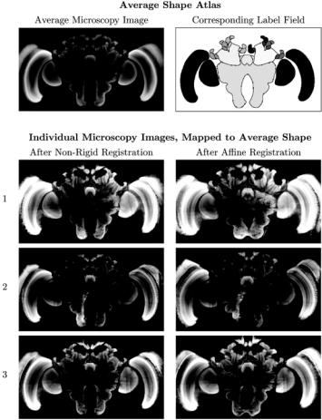
Figure 11.10: Comparison of individual microscopy images and average shape atlas. Note that the average microscopy image of the average shape atlas also has a better signal-to-noise ratio and generally fewer artifacts than the original individual microscopy images (three randomly selected examples shown as rows 1 through 3 in this figure).

11.4.3.4 Noise and Artifacts in the Average Atlas

In Fig. 11.10, we compare some individual images that were used to build the average shape atlas with the average shape atlas itself. It is easy to see that, in addition to representing an average shape, the average atlas also comes with an average microscopy image. The latter is easily generated by averaging the gray values of the appropriately deformed original microscopy images. The average

image shows substantially reduced noise and imaging artifacts. It also shows a more homogeneous distribution of the chromophor compared to the individual brains. All these properties can potentially make registration of the atlas to a given raw image easier, and thus may aid in further improving segmentation accuracy.

11.4.4 Multiatlas Segmentation: A Classifier Approach

We can look at an atlas combined with a coordinate mapping from a raw image as a special type of classifier. The input of the classifier is a coordinate within the domain of the raw image. The classifier output, determined internally by transforming that coordinate and looking up the label in the atlas at the transformed location, is the label that the classifier assigns to the given raw image coordinate.

As we have briefly mentioned before, using a different atlas leads to a different segmentation of a given raw image. From a classifier perspective, we can therefore say that different atlases generate different classifiers for the same raw image. In the pattern recognition community, it has been well-known for some time that multiple independent classifiers can be combined, and together consistently achieve classification accuracies, which are superior to that of any of the original classifiers [27].

Successful applications of multiple classifier systems have been reported in recognizing handwritten numerals [30, 83] and in speech recognition [1, 65]. In the medical image analysis field, this principle has been applied, for example, to multi-spectral segmentation [42] and to computer-aided diagnosis of breast lesions [17, 47].

The particular beauty of applying a multiclassifier framework to atlas-based segmentation is that multiple independent classifiers arise naturally from the use of multiple atlases. In fact, multiple classifiers also arise from using the same atlas with a different non-rigid registration method. However, adding an additional atlas is typically easier to do than designing an additional image registration algorithm. One could, however, also apply the same basic registration algorithm with a different regularization constraint weight (see section 11.3.4), which would also lead to slightly different segmentations.

For the demonstration in this chapter, we performed a leave-one-out study with only one registration method, but a population of independent atlases. Each