Kluwer - Handbook of Biomedical Image Analysis Vol

The variations are calculated by taking the Gateaux derivative [25] of the functional U evaluated at ϕ + εη with respect to ε and then letting ε → 0. For general forms of W and U,

12.2.3 Linearization

Equation (12.6) is highly nonlinear and thus an incremental-interative solution method is necessary to obtain the configuration ϕ that satisfies the equation [27]. The most common approach is based on linearization of the equations and an iterative solution using Newton’s method or some variant. Assuming that the solution at a configuration ϕ is known, a solution is sought at some small increment ϕ + u. Here again, u is a variation in the configuration or a virtual displacement. The linearization of Eq. (12.6) at ϕ in the direction

u is:

ness. These 2nd derivative terms (Hessians) describe how small perturbations of the current configuration affect the contributions of W and U to the overall energy of the system.

12.2.4Particular Forms for W and U—Hyperelastic Warping

In Hyperelastic Warping, a physical representation of the template image is deformed into alignment with the target image, which remains fixed in the reference configuration. The scalar intensity field of the template, T, is not changed directly by the deformation, and thus it is represented as T (X). Since the values of S at material points associated with the deforming template change as the template deforms with respect to the target, it is written as S(ϕ). The formulation

uses a Gaussian sensor model to describe the image energy density functional:

λ is a penalty parameter [28] that enforces the alignment of the template model with the target image data. As λ → ∞, (T (X) − S(ϕ))2 → 0, and the image energy converges to a finite value.

Hyperelastic Warping assumes that W is the standard strain energy density function from continuum mechanics that defines the material constitutive behavior. It depends on the right deformation tensor C. The right deformation tensor is independent of rotation and thus hyperelasticity provides an objective (invariant under rotation) constitutive framework, in contrast to linearized elasticity (see below, [29]). With these specific assumptions, Eq. (12.4) takes the form:

The first variation of the first term in Eq. (12.9) yields the standard weak from of the momentum equations for nonlinear solid mechanics (see, e.g., [25]). The first variation of the functional U in Eq. (12.8) with respect to the deformation

ϕ (X) in direction η gives rise to the image-based force term:

This term drives the deformation of the template based on the pointwise difference in the image intensities and the gradient of the target intensity evaluated at material points associated with the template.

A similar computation for the mechanical strain energy term W leads to the

Thus, the forces applied to the physical model of the deforming template due to the differences in the image data are opposed by internal forces that arise from the deformation of the material through the constitutive model. The particular form of W depends on the material and its symmetry (i.e., isotropic, transversely

In the field of computational mechanics, the first two terms in the second line of Eq. (12.15) are referred to as the geometric and material stiffnesses, respectively [1]. The 2nd order tensor representing the image stiffness for Hyperelastic

These three terms form the basis for evaluating the relative influence of the image-derived forces and the forces due to internal stresses on the converged solution to the deformable image registration problem, as illustrated in the following two sections.

12.2.5 Finite Element Discretization

Hyperelastic Warping is based on an FE discretization of the template image. The FE method uses “shape functions” to describe the element shape and the arbitrary variations in configuration over the element domain [34]. In Hyperelastic Warping, an FE mesh is constructed to correspond to all or part of the template image (either a rectilinear mesh, or a mesh that conforms to a particular structure of interest in the template image). The template intensity field T is interpolated to the nodes of the FE mesh. The template intensity field is convected with the FE mesh and thus the nodal values do not change. As the FE mesh deforms, the values of the target intensity field S are queried at the current location of the nodes of the template FE mesh. To apply an FE discretization to Eq. (12.15), an isoparametric conforming FE approximation is introduced for the variations η and ∆u:

where the subscript e specifies that the variations are restricted to a particular element with domain e, and Nnodes is the number of nodes composing each element. Here, ξ , where := {(−1, 1) × (−1, 1) × (−1, 1)} is the bi-unit cube and Nj are the isoparametric shape functions (having a value of “1” at their specific node and varying to “0” at every other node). The gradients of the variation η are discretized as

Where BL and BNL are the linear and nonlinear strain-displacement matrices, respectively, in Voigt notation [1]. With the use of appropriate Voigt notation, the linearized Eq. (12.15) can be written, for an assembled FE mesh, as:

Equation (12.21) is a system of linear algebraic equations. The term in parentheses on the left-hand side is the (symmetric) tangent stiffness matrix. u is the vector of unknown incremental nodal displacements – for an FE mesh of 8-noded hexahedral elements in three dimensions, u has length [8 × 3 × Nel ], Where Nel is the number of elements in the mesh. F ext is the vector of external

forces arising from the differences in the image intensities and gradients in Eq. (12.12), and F int is the vector of internal forces resulting from the stress divergence. The material and geometric stiffnesses combine to give the mechanics regularization stiffness:

Together, the terms in Eq. (12.22) and Eq. (12.23) form the entire tangent stiffness matrix. In our FE implementation, an initial estimate of the unknown incremental nodal displacements is obtained by solving Eq. (12.21) for uand this solution is improved iteratively using a quasi-Newton method [27].

12.2.6 Solution Procedure and Augmented Lagrangian

In the combined energy function in Eq. (12.9), the image data may be treated as either a soft constraint, with the mechanics providing the “truth”, as a hard constraint, with the mechanics providing a regularization, or as a combination. For typical problems in deformable image registration, it is desired to treat the image data as a hard constraint. Indeed, the form for U specified in Eq. (12.8) is essentially a penalty function stating that the template and target image intensity fields must be equal over the domain of interest as λ → ∞. The main problem with the penalty method is that as the penalty parameter λ is increased, some of the diagonal terms in the stiffness matrix KI become very large with respect to others, leading to numerical ill-conditioning of the matrix. This results in inaccurate estimates for K−I 1, which leads to slowed convergence or divergence of the nonlinear iterations.

To circumvent this problem, the augmented Lagrangian method is used [33, 35]. With augmented Lagrangian methods, a solution to the governing equations at a particular computational timestep is first obtained with a relatively small penalty parameter λ. Then the total image-based body forces ∂U/∂ϕ are incrementally increased in a second iterative loop, resulting in progressively better satisfaction of the constraint imposed by the image data. This leads to a stable

algorithm that allows the constraint to be satisfied to a user-defined tolerance. Ill conditioning of the stiffness matrix is entirely avoided.

The Euler-Lagrange equations defined in Eq. (12.13) are modified by the addition of a term that represents the additional image-based force γ due to the augmentation:

The solution procedure involves incrementally increasing γ at each computational timestep and then iterating using a quasi-Newton method [27] until the energy is minimized. In the context of the FE method described above, the augmented Lagrangian update procedure for timestep n + 1 takes the form:

This nested iteration procedure, referred to as the Uzawa algorithm [36, 37), converges quickly in general because the multipliers γ are fixed during the minimization of G . In practice, the augmentations are not performed until the penalty parameter λ has been incremented to the maximum value that can be obtained without solution difficulties due to ill conditioning. At this last timestep, the augmented Lagrangian method is then used to satisfy the constraint to a user defined tolerance (usually TOL = 0.05).

12.2.7Sequential Spatial Filtering to Overcome Local Minima

The solution approach described above follows the local gradient to search for a minimum in the total energy (Eq. 12.4) and therefore it is susceptible to converging to local minima. This means that the registration process may get “stuck” by alignment of local image features that produce forces locking the deformation into a particular configuration. It is often possible to avoid local minima and converge to a global minimum by first registering larger image features,

such as object boundaries and coarse textural detail, followed by registration of fine detail. Sequential low-pass spatial filtering is used to achieve this goal. By evolving the cut-off frequency of the spatial filter over computational time, the influence of fine textural features in the image can be initially suppressed until global registration is achieved. Fine structure can be registered subsequently by gradually removing the spatial filter.

The spatial filter is applied by convolution of the image with a kernel κ(X ).

For the template image field T,

B

where T (X ) and T (X ) are the original image data and the filtered data respectively in the spatial domain; X is a vector containing the material coordinates and Z is the frequency representation of X. An efficient way to accomplish this calculation is through the use of the discrete Fourier transform.

The convolution of the image data T (X) with the filter kernel κ(X) in Eq. (12.26) becomes multiplication of T (Z) with K(Z) in the Fourier domain.

T (Z) is the Fourier transform of T (X) and K(Z) is the Fourier transform of κ(X). This multiplication is applied and then the transform is inverted to obtain the convolved image in the spatial domain as shown below:

Because of the very fast computational algorithms available for applying Fourier transforms, this method is much faster than computing the convolution in image space. In our implementation, a 3-D Gaussian kernel is used [38]:

Here, σ 2, the spatial variance is used to control the extent of blurring while A is a normalizing constant. Note that Eq. (12.28) is only valid for a 3-D vector

X. The user specifies the evolution of the spatial filter over computational time by controlling the mask and variance. In the specific results reported below, the variance was set to a high value and evolved to remove the filtering as the computation was completed (Fig. 12.2).

The practical application of spatial filtering is complicated by the fact that the registration is nonlinear and is computed stepwise during the registration process. At each step in the computational process, the spatial distribution of

Figure 12.2: Sequential spatial filtering. (A) results of a 10 × 10 pixel mask flat blur to suppress the local detail in the original image (D). (B) 5 × 5 mask. (C) 2 × 2 pixel mask, and (D) original image.

the template intensities changes according to the computed deformation field. Therefore, all image operations on the template during the registration process (including spatial filtering techniques) must be performed on the deformed template image, rather than the static template image before deformation. Since, in most cases, the template finite element mesh nodes are not co-located with the template image voxels, the computed deformation field must be interpolated onto the original template image in order to apply the image operations accurately.

12.2.8 Regular Versus Irregular Meshes

Hyperelastic Warping accommodates an FE mesh that corresponds to all or part of the template image. A “regular mesh” is a rectilinear structured mesh that corresponds to the entire image domain. This mesh may be a subsampling of the actual image voxel boundaries. An “irregular” mesh conforms to a particular structure of interest in the template image. The template intensity field T is interpolated to the nodes of the FE mesh. As the FE mesh deforms, the values of the target intensity field S are sampled at the current location of the nodes of the template FE mesh.

Regular meshes are used primarily for nonphysical deformable image problems (Fig. 12.3). Regular meshes are simple to construct and can easily span the entire image space or a specific region of interest. However, since the mesh does not conform to any structure in the template imaged, these analyses are susceptible to element inversion prior to the completion of image registration. Typically, only a single material type is used for the entire mesh.

Figure 12.3: (A) Template and (B) deformed images of a normal mouse brain cross-section with a representation of a regular finite element mesh superimposed upon the image.

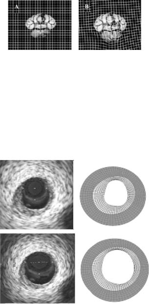
In contrast to regular meshes, irregular meshes are used primarily for physical deformation applications and conform to physical structures of interest in the domain of the image data (Fig. 12.4). Irregular meshes also support the definition of different material models and material properties for specific regions of the mesh. For example, in Fig. 12.4, the irregular mesh represents a cross-section

A B

C D

Figure 12.4: A – intravascular ultrasound cross-sectional image of coronary artery. B – Finite element model of Template image. C – Deformed image of artery after application of 100 mmHg internal pressure load. D – Deformed finite element model after Hyperelastic Warping analysis. The grey area of the arterial wall is represents the intima while the dark gray region represents the adventitia.