Kluwer - Handbook of Biomedical Image Analysis Vol

the segmentation. For the sake of simplicity of the presentation, we assume classifiers that internally use NN interpolation for atlas lookup and therefore only produce one unique label as their output. If the (unknown) ground truth for voxel x is i, we say that x is in class i and write this as x Ci.

11.6.1 A Binary Classifier Performance Model

An EM algorithm described by Warfield et al. [79] estimates the classifier performance for each label separately. The method is based on the common performance parameters p (sensitivity) and q (specificity), i.e., the fractions of true positives and true negatives among the classified voxels. The parameters p and q are modeled independently for each classifier k and each class Ci (label in the segmentation) as the following conditional probabilities:

From these definitions, an EM algorithm that estimates p and q from the classifier decisions can be derived as described by Warfield et al. [79]. From the computed classifier performance parameters for each label, a contradiction-free final segmentation E at voxel x can be computed as

Here, the probability P(x Ci|e) follows from the classifiers’ decisions and their performance parameters using Bayes’ rule. For details on the application of this algorithm to classifier fusion, see [60].

11.6.2 A Multilabel Classifier Performance Model

In a generalization of the Warfield algorithm to multilabel segmentations [60], the classifier parameters p and q are replaced by a matrix of label crosssegmentation coefficients λi(,kj). These describe the conditional probabilities that for a voxel x in class Ci the classifier k assigns label j = ek(x), that is,

This formulation includes the case that i = j, i.e., the classifier decision for that voxel was correct. Consequently, λi(,ki) is the usual sensitivity of classifier k for label i. We also note that for each classifier k the matrix (λi(,kj))i, j is a row-normalized version of the “confusion matrix” [83] in Bayesian multiclassifier

algorithms. This matrix, when filled with proper coefficients, expresses prior knowledge about the decisions of each classifier. Again, the coefficients can be estimated iteratively from the classifier decisions by an EM algorithm.

In the “E” step of the EM algorithm, the unknown ground truth segmentation is estimated. Given the current estimate for the classifier parameters (λ) and the

classifier decisions ek(x), the likelihood of voxel x being in class Ci is

Note that W is a function of two parameters, x and i. The “M” step of our algorithm estimates the classifier parameters (λ) that maximize the likelihood of the current ground truth estimate determined in the preceding “E” step. Given the previous estimates W of the class probabilities, the new estimates for the classifier parameters are computed as follows:

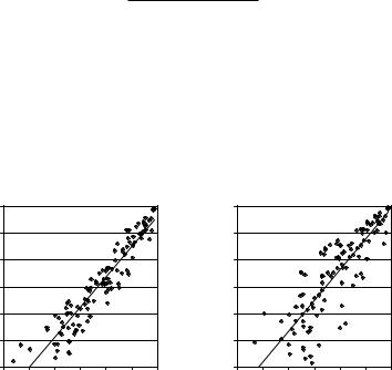
11.6.3Results of Performance-Based Multiatlas Segmentation

The accuracy of the performance parameter estimation using both EM algorithms is shown in Fig. 11.21. We computed the actual performance parameters for each atlas-based classifier by comparing its output with the manual segmen-

Figure 11.21: Accuracy of classifier performance parameter estimation using

EM algorithms.

selection and demonstrated that the accuracy of atlas-based segmentation can be improved substantially by moving beyond the use of a single, individual atlas.

Recently published works on atlas creation and atlas-based segmentation make increasing use of standard atlases that incorporate properties of a population of subjects [33, 35, 45]. Our results confirm that this is likely beneficial for improved segmentation accuracy and robustness. However, our results also suggest that the benefits of applying a multiclassifier strategy are well worth the extra effort.

On a more application-specific note regarding the accuracy of atlas-based segmentation of bee brains, we observe that the mean SI value of segmentations produced using the MUL method in this chapter is 0.86, which, given the small size of most of the structures in the bee brains considered, is comparable to the values reported by Dawant et al. and supports the visual assessment observation (Fig. 11.11) that the automatic segmentations described here differ from manual segmentations on average by slightly more than half of the voxels on the structure surfaces (Fig. 11.14). In fact, Zijdenbos et al. [87] state that “SI > 0.7 indicates excellent agreement” between two segmentations. This criterion (SI > 0.7) is satisfied by virtually all (97%) contours generated by our segmentations using the MUL method (Fig. 11.19). Furthermore, since the image quality of confocal microscopy images is inferior to clinical MR and CT images in many ways, we believe that our registration-based segmentation method represents a satisfactory intermediate solution to a segmentation problem that is appreciably harder than that of segmenting commonly used images of the human brain.

Acknowledgments

Torsten Rohlfing was supported by the National Science Foundation under Grant No. EIA-0104114. While performing the research described in this chapter, Robert Brandt was supported by BMBF Grant 0310961. Daniel B. Russakoff was supported by the Interdisciplinary Initiatives Program, which is part of the Bio-X Program at Stanford University, under the grant “Image-Guided Radiosurgery for the Spine and Lungs.” All computations were performed on an SGI Origin 3800 supercomputer in the Stanford University Bio-X core facility for Biomedical Computation. The authors would like to thank Andreas Steege and Charlotte Kaps for tracing the microscopy images.

Questions

1.What are the advantages of atlas-based segmentation over other segmentation techniques?

2.Why is the described non-rigid registration method superior to other techniques?

3.What is the best value for the smoothness constraint weight of the non-rigid registration (section 11.3.4)?

4.What if in section 11.4.2 the atlas most similar to the raw image were selected using the following criterion I invented: . . . ?

5.When combining multiple atlas-based segmentations, what is the practical difference between NN interpolation with vote fusion and PVI with sum fusion?

6.If the MUL atlas selection strategy is so much better than the others, then why is it not always used?

7.How does atlas-based segmentation compare to manual segmentation?

8.Are there parallels to the multiatlas segmentation method in pattern recognition?

9.Could an active shape model be used as an atlas for segmentation?

10.Why does the binary classifier performance model predict actual performance more accurately, yet the multilabel performance model gives better combined classification results?

Bibliography

[1]Altincay, H. and Demirekler, M., An information theoretic framework for weight estimation in the combination of probabilistic classifiers for speaker identification, Speech Communication, Vol. 30, No. 4, pp. 255– 272, 2000.

[2]Ashburner, J., Computational Neuroanatomy, Ph.D. Dissertation, University College London, 2000.

[3]Baillard, C., Hellier, P. and Barillot, C., Segmentation of brain 3D MR images using level sets and dense registration, Medical Image Analysis, Vol. 5, No. 3, pp. 185–194, 2001.

[4]Bookstein, F. L., Principal warps: Thin-plate splines and the decomposition of deformations, IEEE Transactions on Pattern Analysis and Machine Intelligence, Vol. 11, No. 6, pp. 567–585, 1989.

[5]Online: http://www.bic.mni.mcgill.ca/brainweb/.

[6]Breiman, L., Bagging predictors, Machine Learning, Vol. 24, No. 2, pp. 123–140, 1996.

[7]Bucher, D., Scholz, M., Stetter, M., Obermayer, K. and Pfluger,¨ H.-J., Correction methods for three-dimensional reconstructions from confocal images: I. tissue shrinking and axial scaling, Journal of Neuroscience Methods, Vol. 100, pp. 135–143, 2000.

[8]Cheng, P. C., Lin, T. H., Wu, W. L., and Wu, J. L., eds., Multidimensional Microscopy, Springer-Verlag, New York, 1994.

[9]Christensen, G. E. and Johnson, H. J., Consistent image registration, IEEE Transactions on Medical Imaging, Vol. 20, No. 7, pp. 568–582, 2001.

[10]Christensen, G. E., Rabbitt, R. D. and Miller, M. I., Deformable templates using large deformation kinematics, IEEE Transactions on Image Processing, Vol. 5, No. 10, pp. 1435–1447, 1996.

[11]Collins, D. L. and Evans, A. C., Animal: Validation and applications of nonlinear registration-based segmentation, International Journal of Pattern Recognition and Artificial Intelligence, Vol. 11, No. 8, pp. 1271– 1294, 1997.

[12]Collins, D. L., Holmes, C. J., Peters, T. M. and Evans, A. C., Automatic 3D model—based neuroanatomical segmentation, Human Brain Mapping, Vol. 3, No. 3, pp. 190–208, 1995.

[13]Collins, D. L., Zijdenbos, A. P., Kollokian, V., Sled, J. G., Kabani, N. J., Holmes, C. J. and Evans, A. C., Design and construction of a realistic digital brain phantom, IEEE Transactions on Medical Imaging, Vol. 17, No. 3, pp. 463–468, 1998.

[14]Cootes, T. F., Taylor, C. J., Cooper, D. H. and Graham, J., Active shape models—Their training and application, Computer Vision and Image Understanding, Vol. 61, No. 1, pp. 38–59, 1995.

[15]Crum, W. R., Scahill, R. I. and Fox, N. C., Automated hippocampal segmentation by regional fluid registration of serial MRI: Validation and application in Alzheimer’s Disease, NeuroImage, Vol. 13, No. 5, pp. 847– 855, 2001.

[16]Dawant, B. M., Hartmann, S. L., Thirion, J. P., Maes, F., Vandermeulen, D. and Demaerel, P., Automatic 3D segmentation of internal structures of the head in MR images using a combination of similarity and freeform transformations: Part I, methodology and validation on normal subjects, IEEE Transactions on Medical Imaging, Vol. 18, No. 10, pp. 909–916, 1999.

[17]De Santo, M., Molinara, M., Tortorella, F. and Vento, M., Automatic classification of clustered microcalcifications by a multiple expert system, Pattern Recognition, Vol. 36, No. 7, pp. 1467–1477, 2003.

[18]Forsey, D. R. and Bartels, R. H., Hierarchical B-spline refinement, ACM SIGGRAPH Computer Graphics, Vol. 22, No. 4, pp. 205–212, 1988.

[19]Frangi, A. F., Rueckert, D., Schnabel, J. A. and Niessen, W. J., Automatic 3D ASM construction via atlas-based landmarking and volumetric elastic registration, In: Insana, Information Processing in Medical Imaging:

17th International Conference, IPMI 2001, Insana, M. F. and Leahy, R. M., eds., Davis, CA, USA, June 18–22, 2001, Proceedings, Vol. 2082 of Lecture Notes in Computer Science, pp. 78–91, Springer-Verlag, Berlin Heidelberg, 2001.

[20]Frangi, A. F., Rueckert, D., Schnabel, J. A. and Niessen, W. J., Automatic construction of multiple-object three-dimensional statistical shape models: application to cardiac modeling, IEEE Transactions on Medical Imaging, Vol. 21, No. 9, pp. 1151–1166, 2002.

[21]Gee, J. C., Reivich, M. and Bajcsy, R., Elastically deforming a threedimensional atlas to match anatomical brain images, Journal of Computer Assisted Tomography, Vol. 17, No. 2, pp. 225–236, 1993.

[22]Guimond, A., Meunier, J. and Thirion, J.-P., Average brain models: A convergence study, Computer Vision and Image Understanding, Vol. 77, No. 2, pp. 192–210, 2000.

[23]Hartmann, S. L., Parks, M. H., Martin, P. R. and Dawant, B. M., Automatic 3D segmentation of internal structures of the head in MR images using a combination of similarity and free-form transformations: Part II, validation on severely atrophied brains, IEEE Transactions on Medical Imaging, Vol. 18, No. 10, pp. 917–926, 1999.

[24]Iosifescu, D. V., Shenton, M. E., Warfield, S. K., Kikinis, R., Dengler, J., Jolesz, F. A. and McCarley, R. W., An automated registration algorithm for measuring MRI subcortical brain structures, NeuroImage, Vol. 6, No. 1, pp. 13–25, 1997.

[25]Kikinis, R., Shenton, M. E., Iosifescu, D. V., McCarley, R. W., Saiviroonporn, P., Hokama, H. H., Robatino, A., Metcalf, D., Wible, C. G., Portas, C. M., Donnino, R. M. and Jolesz, F. A., A digital brain atlas for surgical planning, model-driven segmentation, and teaching, IEEE Transactions on Visualization and Computer Graphics, Vol. 2, No. 3, pp. 232–241, 1996.

[26]Kittler, J. and Alkoot, F. M., Sum versus vote fusion in multiple classifier systems, IEEE Transactions on Pattern Analysis and Machine Intelligence, Vol. 25, No. 1, pp. 110–115, 2003.

[27]Kittler, J., Hatef, M., Duin, R. P. W. and Matas, J., On combining classifiers, IEEE Transactions on Pattern Analysis and Machine Intelligence, Vol. 20, No. 3, pp. 226–239, 1998.

[28]Klagges, B. R. E., Heimbeck, G., Godenschwege, T. A., Hofbauer, A., Pflugfelder, G. O., Reifegerste, R., Reisch, D., Schaupp, M. and Buchner, E., Invertebrate synapsins: a single gene codes for several isoforms in Drosophila, Journal of Neuroscience, Vol. 16, pp. 3154–3165, 1996.

[29]Kovacevic, N., Lobaugh, N. J., Bronskill, M. J., B., L., Feinstein, A. and Black, S. E., A robust method for extraction and automatic segmentation of brain images, NeuroImage, Vol. 17, No. 3, pp. 1087–1100, 2002.

[30]Lam, L. and Suen, C. Y., Optimal combinations of pattern classifiers, Pattern Recognition Letters, Vol. 16, No. 9, pp. 945–954, 1995.

[31]Lee, S., Wolberg, G. and Shin, S. Y., Scattered data interpolation with multilevel B-splines, IEEE Transactions on Visualization and Computer Graphics, Vol. 3, No. 3, pp. 228–244, 1997.

[32]Lester, H., Arridge, S. R., Jansons, K. M., Lemieux, L., Hajnal, J. V. and Oatridge, A., Non-linear registration with the variable viscosity fluid algorithm, In: Kuba, Information Processing in Medical Imaging: 16th International Conference, IPMI’99, Visegrad,´ Hungary, June/July 1999. Proceedings, A., Samal, M. and Todd-Pokvopek, A., eds., Vol. 1613, pp. 238–251, Springer-Verlag, Heidelberg, 1999.

[33]Li, B., Christensen, G. E., Hoffman, E. A., McLennan, G. and Reinhardt, J. M., Establishing a normative atlas of the human lung: Intersubject warping and registration of volumetric CT images, Academic Radiology, Vol. 10, No. 3, pp. 255–265, 2003.

[34]Lorenz, C. and Krahnstover,¨ N., Generation of point-based 3D statistical shape models for anatomical objects, Computer Vision and Image Understanding, Vol. 77, pp. 175–191, 2000.

[35]Lorenzo-Valdes,´ M., Sanchez-Ortiz, G. I., Mohiaddin, R. and Rueckert, D., Atlas-based segmentation and tracking of 3D cardiac MR images using non-rigid registration, In: Medical Image Computing and ComputerAssisted Intervention—MICCAI 2002: 5th International Conference,

Tokyo, Japan, September 25–28, 2002, Proceedings, Part I, Dohi, T. and Kikinis, R., eds., Vol. 2488 of Lecture Notes in Computer Science, pp. 642–650, Springer-Verlag, Heidelberg, 2002.

[36]Maes, F., Collignon, A., Vandermeulen, D., Marchal, G. and Suetens, P., Multimodality image registration by maximisation of mutual information, IEEE Transactions on Medical Imaging, Vol. 16, No. 2, pp. 187–198, 1997.

[37]Malladi, R., Sethian, J. A. and Vemuri, B. C., Shape modelling with front propagation: A level set approach, IEEE Transactions on Pattern Analysis and Machine Intelligence, Vol. 17, No. 2, pp. 158–175, 1995.

[38]Miller, M. I., Christensen, G. E., Amit, Y. and Grenander, U., Mathematical textbook of deformable neuroanatomies, Proceedings of the National Academy of Sciences of the U.S.A., Vol. 90, No. 24, pp. 11944– 11948, 1993.

[39]Mobbs, P. G., Brain structure, in Kerkut, G. A. and Gilbert, L. I., eds., Comprehensive insect physiology biochemistry and pharmacology, Vol. 5: Nervous system: structure and motor function, pp. 299–370, Pergamon Press, Oxford, New York, Toronto, Sydney, Paris, Frankfurt, 1985.

[40]Mortensen, E. N. and Barrett, W. A., Interactive segmentation with intelligent scissors, Graphical Models and Image Processing, Vol. 60, No. 5, pp. 349–384, 1998.

[41]Musse, O., Heitz, F. and Armspach, J.-P., Fast deformable matching of 3D images over multiscale nested subspaces. application to atlas-based MRI segmentation, Pattern Recognition, Vol. 36, No. 8, pp. 1881–1899, 2003.

[42]Paclik, P., Duin, R. P. W., van Kempen, G. M. P. and Kohlus, R., Segmentation of multispectral images using the combined classifier approach, Image and Vision Computing, Vol. 21, No. 6, pp. 473–482, 2003.

[43]Park, H., Bland, P. H. and Meyer, C. R., Construction of an abdominal probabilistic atlas and its application in segmentation, IEEE Transactions on Medical Imaging, Vol. 22, No. 4, pp. 483–492, 2003.