

Kluwer - Handbook of Biomedical Image Analysis Vol
.3.pdfSource MR image Target MR image
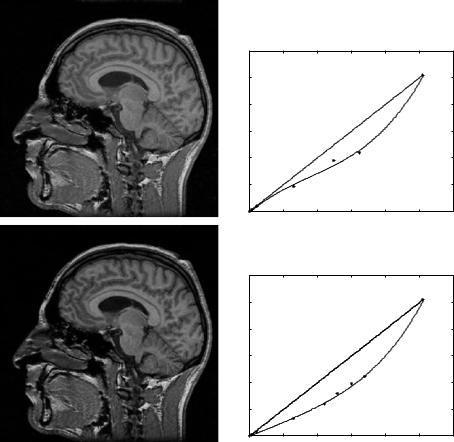
Figure 8.4: MR images of different subjects. The intensity of tissue classes is different for source (top) and target (bottom) volume.
300 |
|
|
|
|
|
|
250 |
|
|
|
|
|
|
200 |
|
|
|
|
|
|
150 |
|
|
|
|
|
|
100 |
|
|
|
|
|
|
50 |
|
|
|
|
|
|
0 |
50 |
100 |
150 |
200 |
250 |
300 |
0 |
300 |
|
|
|
|
|
|
250 |
|
|
|
|
|
|
200 |
|
|
|
|
|
|
150 |
|
|
|
|
|
|
100 |
|
|
|
|
|
|
50 |
|
|
|
|
|
|
0 |
50 |
100 |
150 |
200 |
250 |
300 |
0 |
Figure 8.5: Intensity correction using the expectation maximization (EM) algorithm. The corrected source volume is presented, as well as the parametric intensity correction (to be compared with the identity function). The histogram has been modeled by five Gaussian distributions (top) and seven Gaussian distributions (bottom). Points represent the mean of Gaussian laws that model the histogram.
300 |
Hellier |
300 |
|
|
|
|
|
|
250 |
|
|
|
|
|
|
200 |
|
|
|
|
|
|
150 |
|
|
|
|
|
|
100 |
|
|
|
|
|
|
50 |
|
|
|
|
|
|
0 |
50 |
100 |
150 |
200 |
250 |
300 |
0 |
300 |
|
|
|
|
|
|
250 |
|
|
|
|
|
|
200 |
|
|
|
|
|
|
150 |
|
|
|
|
|
|
100 |
|
|
|
|
|
|
50 |
|
|
|
|
|
|
0 |
50 |
100 |
150 |
200 |
250 |
300 |
0 |
Figure 8.6: Intensity correction using the stochastic expectation maximization (SEM) algorithm. The corrected source volume is presented, as well as the parametric intensity correction (to be compared with the identity function). The histogram has been modeled by five Gaussian distributions (top) and seven Gaussian distributions (bottom). Points represent the mean of Gaussian laws that model the histogram.
Corrected source volumes and parametric correction functions are presented. The corrected volume seems visually more similar to the target volume (when comparing intensities of corresponding tissues). Modeling the histogram with seven classes seems more adequate in this context. This is actually more relevant from an anatomical point of view and provides more sample to estimate the correction function. The experiments we have conducted so far do not
Inter-Subject Non-Rigid Registration |
301 |
Before correction |
After correction |
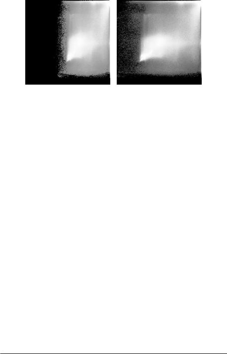
Figure 8.7: Joint histogram before and after intensity correction. To compute the joint histogram, MR volumes have been previously rigidly registered by maximizing mutual information [88].
favor the SEM or the EM algorithm. There may be an indication that the SEM is more adapted in presence of field inhomogeneity and should be investigated further.
The relevance of this intensity correction can be assessed using the joint histogram (Fig. 8.7). To compute the joint histogram, a spatial alignment of the volumes needs to be performed. To do so, we estimate a rigid displacement that maximizes mutual information [88]. Figure 8.7 shows the joint histogram before and after intensity correction (using EM and seven Gaussian laws to model the histogram). It must be noted that the same displacement has been applied to the corrected and uncorrected volume (in other words, the effect of a possible misalignment is equal for both histograms). The joint histogram shows the relevance of the intensity correction.
8.3.3.2 Experiments on Simulated Data
Evaluation on the MNI Phantom. To evaluate the global registration method, we use the simulated data provided by the MNI3 [34]. Data have been collected with three levels of noise and inhomogeneity. We design a synthetic deformation field made up of a global affine field with large deformations combined with local stochastic perturbations. We do not try to build a “realistic”
3 Brainweb: http://www.bic.mni.mcgill.ca/brainweb

302 |
Hellier |
field, but rather a field with the following properties: large deformations and local perturbations that modify the topology of the structures, in order to validate the basic hypothesis of our work. The “local” field is generated from 2,000 voxels which are randomly picked in the volume. For each voxel, each of the three components of the deformation is the realization of a Gaussian random variable of standard deviation 120 mm. We then perform a Gaussian smoothing with a small average deviation in order to propagate this perturbation to a local neighborhood while preserving discontinuities. The volumes and the results are shown on Fig. 8.8. We compare the multigrid method with a global affine registration method, in which a 12-parameter deformation is estimated for the entire volume.
To asses the quality of the registration, we compute the mean square error (MSE)4 which is an indicator of the quality of the registration. However, it would be unfair to evaluate the registration only with a measure that is the underlying driving force of the estimation. Therefore, as we have the binary classification of the phantom, we can also assess the quality of the registration based on the overlap of two volumes: the first volume is the initial classification, i.e., a gold standard (gray matter/white matter), the second volume is the deformed classification, registered with the estimated deformation field. We then measure out overlapping ratios like the sensitivity, the specificity, and the total performance [142]. Results are presented in Table 8.1. Despite the use of binary classes, the resulting measures that we obtain are very satisfactory. Particularly, the robustness of the method is demonstrated in critical conditions (9% noise and 40% inhomogeneity), which are far tougher than in any realistic acquisition.
The numerical evaluation also allows to study the sensitivity of the algorithm with respect to the parameters of the algorithm, i.e., parameters of the robust estimators. We have two parameters to fix, σ1 and σ2. σ1 corresponds to the hyperparameter of robust function ρ1, associated with the similarity term, while
σ2 corresponds to the hyperparameter of robust function ρ2 associated with the regularization term. We made the parameters σ1 and σ2 vary in a cube of size [1.0e4, 1.0e5] × [1, 20] with step, respectively, of 1.0e4 and 1 (which means that we performed the registration with 200 different sets of parameters), and we observe that the final result (the mean square error between the source volume
4 |
|
|
1 |
i=N |
|
2 |
|
|
|
M SE = |
N |
i=1 |
(I1 |
(i) − I2(i)) |
, where I1 |
and I2 are the volumes to compare, and N is |
|
the number of |
voxels. |
|
|
|
||||
|
|
|
|
|
|
|||
Inter-Subject Non-Rigid Registration |
303 |
Original data
original phantom |
deformed with the synthetic field |
Reconstructed volumes
Global affine registration |
Non-linear robust registration |
Difference volumes
Global affine registration |
Multigrid robust registration |
Figure 8.8: Results of the registration process on simulated data. The 3D MRI phantom has been deformed on the top of the figure. In the middle, the reconstructed volumes are shown and must be compared with the initial volume to evaluate the quality of the registration. On the bottom, the difference volumes show the benefits of non-linear registration.
and the reconstructed volume) varies less than 5% of the nominal MSE. This indicates that the sensitivity of algorithm with respect to these two parameters is very low.
For simulated data, mean square error (MSE) is a direct measure of the quality of the registration. Therefore we can also evaluate the influence of f (see section 8.3.2) on the computation time and on the accuracy of the registration.

304
Table 8.1: Objective measures of the quality of the registration on simulated data. Specificity, sensitivity and total performance measures are given for three levels of noise and two registration methods. The registration processes are performed until resolution 0 (voxel size 1 mm3). We manage to recover up to 93% of the deformation even in presence of important noise (9%) and image intensity inhomogeneity (40%). The CPU times are given for an Ultra Sparc at 333 Mhz
|
|
Noise |
0% |
|
Noise |
3% |
|
Noise |
9% |
|
|
|
Inhomogeneity |
0% |
|
Inhomogeneity |
20% |
|
Inhomogeneity |
40% |
|
|
|
Target |
Grey |
White |
Target |
Grey |
White |
Target |
Grey |
White |
|
|
volume |
matter |
matter |
volume |
matter |
matter |
volume |
matter |
matter |
|
|
|
|
|
|
|
|
|
|
|
|
Computation time |
10 |
|
|
10 |
|
|
10 |
|
|
|
MSE |
964.63 |
2679.49 |
1751.41 |
1104.22 |
3305.50 |
2171.13 |
2005.14 |
6933.05 |
5031.49 |
Global |
sensitivity |
|
93.78% |
91.19% |
|
93.26% |
89.01% |
|
83.21% |
77.33% |
affine |
specificity |
|
93.16% |
93.72% |
|
91.69% |
92.48% |
|
83.19% |
85.42% |
|
total performance |
55 |
93.27% |
93.41% |
61 |
91.97% |
92.06% |
76 |
83.19% |
85.42% |
|
Computation time |
|
|
|
|
|
|
|||
|
MSE |
138.57 |
1383.46 |
886.53 |
233.23 |
1534.48 |
970.42 |
667.88 |
3186.49 |
1463.87 |
Robust |
sensitivity |
|
97.83% |
97.35% |
|
97.09% |
96.36% |
|
95.50% |
93.27% |
multigrid |
specificity |
|
94.28% |
94.35% |
|
94.76% |
94.90% |
|
90.73% |
93.67% |
|
total performance |
|
94.91% |
94.71% |
|
95.35% |
95.03% |
|
91.50% |
93.80% |
|
|
|
|
|
|
|
|
|
|
|
Hellier
Inter-Subject Non-Rigid Registration |
305 |
|
550 |
|
|
|
initialization with |
|
500 |
result of resolution 1 |
|
450 |
|
MSE |
400 |
|
|
|
|
|
350 |
|
300
250
5 |
4 |
3 |
2 |
1 |
0 |
GRID LEVEL
MSE
COMPUTATION TIME
70
60
50
40
initialization with
result of resolution 1
30
20
10
5 |
4 |
3 |
2 |
1 |
0 |
GRID LEVEL
Computation time
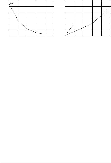
Figure 8.9: Evolution of the MSE with respect to the grid level (at finest resolution 1 mm) and computation time needed to perform the registration until a given grid level. We observe that the MSE decreases significantly at the coarsest grid level, whereas at the finest grid level it continues to decrease, but less rapidly. At the same time, the computation time increases continuously. If we look at the difference between grid level 2 (the smallest cubes are of size 22 × 22 × 22 and the incremental deformation field is affine on each cube) and grid level 0 (the smallest cubes are reduced to a voxel and the incremental deformation field is translational for the smallest cubes), the computation time increases by 100%, whereas the MSE variation is only 5.3%. That suggests that, depending on the application, the user can make a compromise between the accuracy of the registration and the computation time if the resources are limited.
Figure 8.9 shows the evolution of the MSE with respect to the grid level (at finest resolution 1 mm) and also shows the computation time needed to perform the registration until a given grid level. We observe that the MSE decreases significantly at coarsest grid level, whereas at the finest grid level it continues to decrease, but less rapidly. At the same time, the computation time increases continuously. If we look at the difference between grid level5 2 and grid level6 0, the computation time increases by 100%, whereas the MSE variation is only 5.3%. That suggests that, depending on the application, the user can make a compromise between the accuracy of the registration and the computation time
5 The smallest cubes are of size 22 × 22 × 22 and the increment deformation field is affine
on each cube.
6 The smallest cubes are reduced to a voxel and the increment deformation field is translational for the smallest cubes.

306 |
Hellier |
Source volume |
Target volume |
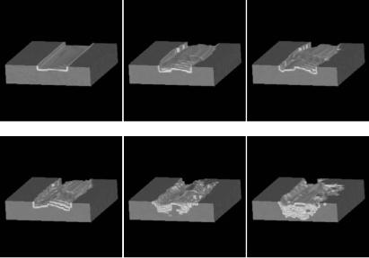
Figure 8.10: Synthetic data to validate the link between robust estimator on the regularization term and local changes of topology.
if its resources are limited. In our case, we find that f = 1 (the smallest cubes are of size 2 × 2 × 2 and the allowed deformation is rigid on the smallest cube) is generally a good compromise.
Importance of Robust Estimator. We have introduced robust estimators in the registration process, in order to let local discontinuities of the deformation field occur. We now want to verify on simulated data the direct link between the introduction of a robust function and the possibility to locally change the topology of the structures. Therefore, we construct two volumes (see Fig. 8.10) to be registered, with a local modification of the topology. The volumes are composed of two homogenous classes, each one being defined by a unique gray level. With these two volumes, we obviously face the aperture problem, which is classical in the optical flow literature.
We first register the two volumes without any robust estimator. Results are presented in Fig. 8.11. The reconstructed volumes are computed with the target volume and the estimated deformation field with trilinear interpolation. One must therefore compare the reconstructed volume and the source volume to assess the quality of the registration. The different volumes shown in Fig. 8.11 correspond to different values of the parameter α. This parameter balances the importance of the similarity term and the regularization term. When this parameter is high, the solution is smooth but the topology is not modified. When α decreases, the solution is not smooth, the aperture problem is obvious, whereas the topology is not correctly modified.
Inter-Subject Non-Rigid Registration |
307 |
a = 5000 |
a = 1000 |
a = 500 |
a = 250 |
a = 100 |
a = 50 |
Figure 8.11: Results of the registration without robust estimator. The different volumes correspond to different values of the parameter α, and must be compared to the source volume.
We then perform the robust multigrid registration process, with a robust function only on the regularization term. Results are presented in Fig. 8.12, with two “extreme” values of the parameter α. In that case, the modification of the topology is possible, while preserving the global smoothness of the solution. However, the aperture problem is still present in the tubular structure on the right. This experiment makes it possible to verify the link between the introduction of a robust estimator on the regularization term and the possibility to handle local change of topology. In addition, the robust registration process appears to be also more robust with respect to the parameter α, because the results of the registration are very similar, when α varies in a range of [100, 3,000].
8.3.3.3 Experiment on Two Subjects
Importance of Intensity Correction. We first want to present cases where the registration method cannot work properly without a prior intensity

308 |
Hellier |
a = 100 |
a = 3000 |
Figure 8.12: Results of the registration with a robust estimator on the regularization term. The reconstructed volumes must be compared to the source volume. We can handle with local topology changes, while preserving the global smoothness of the solution.
correction. Figure 8.13 shows the impact of the intensity correction step on the registration of two volumes. The source image is first corrected using the EM algorithm, seven classes to model the histogram and a fourth order parametric correction. Figure 8.13 presents the source image deformed toward the target image, as well as the difference image. While the registration has failed without intensity correction due to a very large intensity difference, it has performed successfully with an intensity correction step. It must be noted that the set of parameters is the same for both registration processes. That demonstrated the usefulness of such correction for a non-rigid registration task.
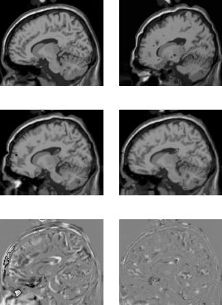
Extensive Results for Two Subjects. Results of the 3D method are presented in Figs. 8.14, 8.15, and 8.16. Two 3D MRI-T1 volumes of two different subjects are registered. The source volume, the target volume and the reconstructed volume are presented in Fig. 8.14. The reconstructed volume f2(s + wˆ s) is computed with the target volume f2 and the final displacement field wˆ by the way of a trilinear interpolation. To assess the quality of the registration, one must compare the source volume with the reconstructed volume.
We also present the volumes of difference, before and after registration in Fig. 8.15. In the same figure, the adaptive partition at grid level 3 is also presented (we do not present further grid levels for readability reasons). The difference volumes must be interpreted carefully, since we get the superposition of two