Kluwer - Handbook of Biomedical Image Analysis Vol

−→

where κ is the mean curvature of the evolving surface and n is its outer unitary normal vector. So, the evolution of the surface is driven by the associated gradient descent equation

Following this equation, the surface evolves toward the minimum of the functional, which is achieved at the edges of the image. The resulting steadystate surface is a model of the object of interest. The level set method [29] is used to track its motion, allowing topological changes in the surface and avoiding numerical instabilities. Basically, the level set method consists in embedding the evolving surface in a manifold one dimension higher than S, and implicitly represented by a function φ. The surface S can be reconstructed as the level set

then the evolution of the zero level set of φ is equivalent to the evolution of S driven by Eq. (5.9).

5.2.4.2Introduction of Region-Based Information in the GAC Model

The GAR model [19] combines the classical GAC model [27] with region-based statistical information incorporated into the classical energy functional. Therefore, in places where the gradient is weak, regional information drives the evolution of the surface thus being more robust than GAC.

A surface S provides a partition of the space in three regions: inside ( in), outside ( out), and the boundary itself (S). Considering the surface evolving in the domain of a three-dimensional image, the surface provides the following partition at each time:

Given a partition of the image domain defined by S(t), the descriptor of the inner region is defined as

where Pin is the probability for a voxel x to belong to in. An analogous definition holds for the outer region.

Following the ideas of the theory of GAC, the energy functional associated

to the region-based model is defined as

E(t) = ζ kin(x; t) dx + ζ kout(x; t) dx + η g(x)da (5.13)

in (t) out (t) S(t)

where ζ and η control the contribution of the regional and boundary information, respectively.

The evolution of the regions in which the domain is divided can be simplified by expressing it in terms of the evolution of the boundary S(t). So the evolution

can be expressed by the partial differential equation

∂ S(x; t)

(5.14)

∂t

where F(x; t) is the evolution speed.

The gradient descent flow associated to the minimization of the functional

As region descriptors, we propose to use the negative logarithm of the probabilities learned from the kNN rule. When using multiple features, like in our approach, a non-linear PDF estimation technique can better adapt to the distributions of the underlying tissues than the traditionally used Gaussian PDFs. So, the probability of the inner region is computed as

and kNN descriptors, it can be shown that these terms have zero contribution (see [16] for the case of Gaussian descriptors).

The outer probability combines the region information of the bone and background tissues. If we assume this distributions to be independent (i.e.,

C1 ∩ C2 = ), then

Pout = P(I(x) = i|C1 C2) = P(I(x) = i|C1) + P(I(x) = i|C2) (5.18)

5.2.4.3 Considerations of Implementation

kNN Algorithm. For the construction of the classifier, six images were selected, and a total of N = 1830 points were manually picked and labelled. Image features were computed with a Gaussian aperture of σ = 0.8 mm. In our approach, we used k = 10 as size of the kNN neighborhood.

For the-extraction of the nearest neighbors, a brute-force computation is highly time-consuming, specially if the size of the training set or the dimension of the feature vector are large. For this reason, we used the approximate nearest neighbors (ANN) algorithm [30], that computes efficiently the k- nearest neighbors from a given vector. The ANN library implements a number of different data structures, based on kd-trees and box-decomposition trees, and employs different search strategies for speeding-up the search process.

Numerical Schemes for GAR. The level set equation φt = F| φ| is an hyperbolic equation that belongs to the family of Hamilton-Jacobi equations. Only in one dimension, the level set equation is an hyperbolic conservation law. Nevertheless, the numerical methodology developed to solve conservation laws can be generalized to obtain numerical schemes that solve Hamilton-Jacobi equations and, in particular, the level set Equation [31]. The Courant-Friedrichs-Levy (CFL) condition is used to compute the optimal time step for the GAR level set equation [32]. The term ζ (kout − kin)| φ| represents a motion in the normal direction. An upwind numerical scheme is used to select the correct solution. The term gκ| φ| represents a motion involving mean curvature. This term acts as a viscous force so a scheme with central differences is sufficient to select the correct solution. The term g φ represents a motion in an externally generated velocity field. This term is also called advection term. Upwind numerical differences are also used to select the correct solution in this case.

Initialization and Reinitialization with the Fast Marching Method. The Fast Marching algorithm is an efficient method to compute the solution of the Eikonal equation F · | T | = 1 with initial condition T0 = 0. If F = 1, the solution

of the equation is the distance transform to the surface represented by the initial condition, T0 = 0. The initial surface is computed as the boundary vessel voxels in the MAP classification. The Fast Marching algorithm is used to compute the distance transform to this surface. This function is used as initialization to the level set algorithm.

The level set equation, Eq. (5.16), does not preserve the distance transform through the iterations. The numerical approximations described below may cause a numerical deterioration of the solutions if the evolving front φ is not smooth enough. To avoid this phenomenon, φ is replaced in each iteration by a distance transform φ with the same level set zero as φ. To do this, the Fast Marching algorithm is used. The values of the voxels where there is a change of sign define the evolving surface. These voxels are introduced in the Fast Marching algorithm as initial condition instead of explicitly computing the zero level set and then use it as initial condition. The result is also a distance transform to

the evolving surface.

Curvature Constraints. The mean curvature of a surface is defined in differential geometry as the inverse of the radius of the osculant sphere. If the minimum grid size is x, it makes no sense considering osculant spheres of sizes less than x. So, the discrete values of the curvature are limited to the interval [− 1x , 1x ]. The numerical approximation introduces singularities in the calculus of the curvature function. To avoid their propagation in the GAR algo-

rithm, a Gaussian smoothing with σ = 0.8 mm was applied to the curvature.

Parameter Selection. Parameters ζ and η control the influence of the region and boundary based forces in the motion of the surface. The choice of these parameters depends on the confidence of the user in the different descriptors.

For this application, ζ and η were chosen equal to 1.0.

Regarding the selection of the edge detector function g, there is an interesting property that relates the parameters involved in the level set equation to a bound on the curvature of the front in evolution. The front evolution is driven

In the case of segmentation of narrow vessels, the curvature of the model is high at certain locations. Therefore, the selection of the parameters has to be

such that the curvature is not limited by the right-hand term of inequality (5.19). Remember that the curvature was also bounded by 1x , so the resolution of the image grid provides another constraint to the algorithm in the capture of narrow structures.

Traditionally, two functions have been used as contour detectors

where σ I = (I Gσ ) and Gσ is a Gaussian kernel. In this work, the Leclerc function (Eq. (5.21)) was used with σ = 0.8 mm, as edge detector function. For the selection of , we noted that in places where kout ≈ kin, Inequality (5.19) leads to |κ| ≤ || σ I||∞. So if 1 < 2, the steady-state model associated with 2 will be able to capture narrower structures than the steady-state model associated to 1. Therefore, in all the experiments, the Leclerc contour detector function g was selected with = 10. Less than 20 iterations were then enough to assure convergence of the algorithm.

5.3 Evaluation: Materials and Methods

5.3.1 Clinical Protocol

The evaluation study was performed on a data base of 39 brain aneurysms located mostly at the Circle of Willis; more specifically, at the Anterior Communicating (16), Posterior Communicating (10) and Middle Cerebral (10) Arteries. There were also three aneurysms located at the Pericallosal (1) and Internal Carotid Arteries (2). Aneurysm sizes (dome depth size) varied from 2.9 to 16.3 mm. Table 5.1 shows the distribution of sizes, manually measured, according to the location of the aneurysm.

Image acquisition was performed using an Helical Elscint CT Twin scanner (Marconi; Haifa, Israel) with 120 kV/300 mA for the amplifier tube, 1.2-mm collimation with an helical pitch of 1 and slice spacing of 0.65 mm. Images were reconstructed on a 512 × 512 matrix with a square Field Of View (FOV) of 20.8 cm yielding an in-plane resolution of 0.4 mm. A total of 140 ml of non-ionic contrast fluid was intravenously administrated (Omnitrast 300 mg; Schering,

Table 5.1: Overview of aneurysm dimensions present in our database assessed via manual measurements done by a neuroradiologist. The table shows mean ± SD of the mean of the manual measurements by two observers. Aneurysms were stratified according to their location

Berling, Germany) at a rate of 3 ml/s, starting the scanning 20 seconds after the onset of contrast administration.

The acquired images were transferred to a SGI Indigo2 workstation (Silicon Graphics, Mountain View, CA) for viewing and postprocessing. The manual quantification of the aneurysms was performed using 2D MIP images and measuring tools provided by the console software Omnipro (Marconi; Haifa, Israel). The clinical parameters needed for the planning of the endovascular intervention were the maximum neck diameter, the maximum dome width, and maximum dome depth of the aneurysm. As it is customary in clinical routine, the measurements were carried out along several projection angles and, from those, the neuroradiologist chose the view-angle producing maximal measurements.

5.3.2 Computerized Protocol

Using the marching cubes algorithm, a 3D model of the aneurysm was reconstructed from the zero-level set of φ. To make the computerized measurements comparable to the manual gold standard, the models were rendered with a viewpoint selected according to the criterion of maximality used to generate the MIP images. Two points were manually pinpointed in the 3D scene, corresponding to the end-point of the measured magnitude from that angle. Measurements are then performed by projecting this points into the camera plane to emulate MIP-based measurements.

5.4 Results

5.4.1 Examples

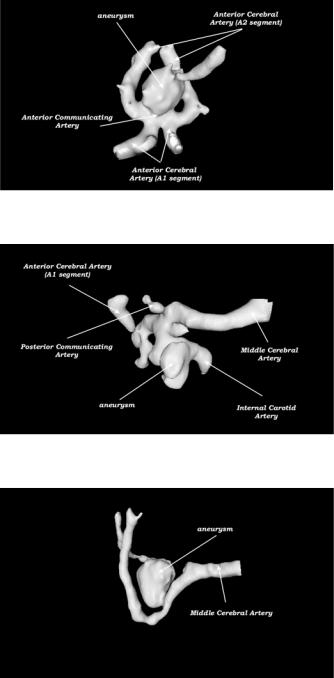
In Fig. 5.8 and 5.9 we show some examples of the segmentations of some representative aneurysms from our data base.

5.4.2 Evaluation

Two experts carried out the manual measurements twice per aneurysm with enough delay between sessions to consider them independent. The average of the manual measurements is considered as gold-standard and compared to the measurements obtained by the model based approach. Analysis of variance is used to estimate the reproducibility of the manual method. Bland–Altman analysis [33] is used to obtain the repeatability of the manual method for each of the two observers, the agreement between the observers, and the agreement between the manual and the computerized method.

5.4.2.1 Analysis of Variance

In the ANalysis Of VAriance (ANOVA) model, measurements are considered samples from a random variable that follows a linear statistical model. The associated variance is factored out into the components of the variance according to

where σS2 is the variance due to inter-subject differences, σO2 is the variability introduced by the observers, σH2 is the variability introduced by the observersubject interaction, and σW2 is the within-subject random variation. The analysis of variance allows to estimate the significance that each component has in their contribution to the total variance of the measurements and the intraand interobserver variation.

A first analysis of variance reported no statistically significant interaction between the observer and the subject (σH ) with p > 0.55 in all cases. The results of the analysis of variance with the suppression of this term are presented in Tables 5.2–5.4. Table 5.5 presents the results of the intraand interobserver variation.