

Kluwer - Handbook of Biomedical Image Analysis Vol
.3.pdfInverse Consistent Image Registration |
229 |
resolution later to get the final transformation. The advantage of solving the problem on a course grid is that the algorithm requires fewer computations per iteration than a finer grid. This results in reduced computation time at low resolution. Each time the resolution of the grid is increased by a factor of two in each dimension, the computation time increases by a factor of eight. The drawback of solving the problem at low resolution is that there can be significant registration errors due to the loss of detail in the down sampling procedure. The trade-off between quicker execution times at low resolution and more accurate registration at higher resolution can be exploited by solving the registration problem at low spatial resolution during the initial iterations to approximate the result and then increasing the spatial resolution to get a more accurate result at the later iterations.
The spatial multiresolution approach works well with the frequency multiresolution approach provided by increasing the number of harmonics used to represent the displacement fields. The number of harmonics used to represent the displacement fields is initially set small and then increased as the number of iterations are increased. A low-frequency registration result is an approximation of the desired high-frequency registration result. Computing the gradient descent for a low-frequency basis coefficient at low spatial resolution gives approximately the same answer as using high spatial resolution but the computational burden is much less.
6.2.8Tracking the Jacobian During the Estimation Procedure
It is important to track both the minimum and maximum values of the Jacobian during the estimation procedure. The Jacobian measures the differential volume change of a point being mapped through the transformation. At the start of the estimation, the transformation is the identity mapping and therefore has a Jacobian of one. If the minimum Jacobian goes negative, the transformation is no longer a one-to-one mapping and as a result folds the domain inside out [31]. Conversely, the reciprocal of the maximum value of the Jacobian corresponds to the minimum value of the Jacobian of the inverse mapping. Thus, as the maximum value of the Jacobian goes to infinity, the minimum value of the Jacobian of the inverse mapping goes to zero.

230 |
Christensen |
Figure 6.2: Notation used to describe transformations from one coordinate system to another.
6.3 Transformation Properties
The following definitions will be used throughout this section. Let Ti for i Q = { A, B, C, . . .} denote a set of homogeneous, topologically-equivalent anatomical images defined on the coordinate system or domain = [0, 1]3. For example,
TA, TB, etc., may correspond to a set of 3D MRI brain images collected from age and sex matched normals or abnormals or some other suitable classification criteria. Let hAB represent the transformation from the coordinate system of image TA to that of image TB in terms of the coordinate system of image TB as shown in Fig. 6.2. Let the linear transformation x = hAB(y) deform image
˜ =
TA(x) into a new image T (y) TA(hAB(y)) that resembles the shape of image
TB(y) by transforming the coordinate system of image TA to that of image TB.
Define H as the set of all transformations h (x) for A, B Q and x . Let
AB
||x|| = x12 + x22 + x32 denote the standard 2-norm.
6.3.1 Invertibility Property
Many nonlinear image registration algorithms have difficulty producing inverse consistent transforms because they use a finite set of basis functions (eigenfunctions of an operator, polynomials, etc.) that are not always closed under composition. This observation is a major reason why it is important to measure the inverse consistency error produced by different registration algorithms. This fact motivates the minimization of the inverse consistency constraint error that is used by the consistent linear elastic registration error since it is not possible to reduce the inverse consistency error to zero when using the a finite set of complex exponential basis functions.
Inverse Consistent Image Registration |
231 |
Another reason why it is difficult to produce inverse consistent transformations is that numerical optimization techniques used to find the optimal image transformation often take a long time to converge or get stuck in local minima. The large number of parameters estimated and the nonlinearity introduced by the images being mapped makes it very difficult to find the optimal transformation. Placing a limit on the acceptable inverse consistency error may be one way
of specifying the stopping criteria for a particular optimization technique.
Formally, |
transformations |
hAB : → and hB A : → are |
said to |
be inverses |
of one another if |
the transformation hB A exists and |
satisfies |
hAB(hB A(x)) = x and hB A(hAB(x)) = x for all x . A set of linear transformations H is said to have the invertibility property if hAB(hB A(x)) = x for all
A, B Q and x .
The average Inverse Consistency (IC) error within a region of interest (ROI)
M is defined as
1 |
M |
|
|
|
|
|
EAIC (hAB, hB A, M) = |
|
||hAB(hB A(x)) − x||dx |
(6.6) |
|||
M |
||||||
and the maximum IC error is defined as |
|
|
|
|
||
EM IC (hAB, hB A, M) = x M |
||hAB |
hB A |
x − x||. |
(6.7) |
||
|
max |
( |
( |
)) |
||
Eqs. (6.6 and 6.7) are discretized for implementation.
It is important to define a ROI because the amount of padding applied to the image data can have a significant effect on the average error calculation. The ROI restricts the error measurements to areas of interest preventing the situation where the largest error occurs in the background of the image.
6.3.2 Transitivity Property
Image registration algorithms that have a difficult time producing inverse consistent transformations have an even harder time producing transformations that satisfy the transitivity property. In the paper we investigate how an algorithm that reduces the inverse consistency error compared to another also reduces the transitivity error.
A set of image transformations H is said to have the transitivity property if hC B(hB A(x)) = hC A(x) or equivalently if hAC (hC B(hB A(x))) = x for all A, B, C Q and x .
232 Christensen
These transitivity relationships are illustrated in Fig. 6.2. Assume that
the points x, y, and z correspond to the same landmark in |
images A, |
B, and C, respectively. Assume that the set of transformations |
H = {hAB, |
hB A, hBC , hCB, hAC , hCA} has the invertibility and transitivity properties such that
y = hB A(x), z = hCB(y), x = hAC (z).
Substituting the first equation into the second and the second into the third equation gives the result
x = hAC (hCB(hB A(x))). |
|
||||
The average transitivity error is defined as |
|
|
|
||
1 |
M ||hAB(hBC (hCA(x))) − x||dx |
|
|||
EATRAN(hAB, hBC, hCA, M) = |
|
(6.8) |
|||
M |
|||||
and the maximum transitivity error is defined as |
|
|
|
||
EM T RAN (hAB, hBC , hC A, M) = x M ||hAB |
( |
hBC (hC A(x))) − x||. |
(6.9) |
||
|
|
max |
|
||
Equations (6.8) (6.9) are discretized for implementation.
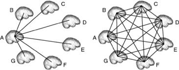
Figure 6.3 demonstrates an advantage of producing transformations that satisfy the transitivity property. The left panels show that the minimum number of invertible transformations required to map information from one coordinate system to another is N − 1 where N is the number of image volumes. The
Figure 6.3: The left panel shows the minimum number of pairwise transformations needed to map a point from one brain to its corresponding location in another. The right panel shows all of the pairwise mappings between the brains.
Inverse Consistent Image Registration |
233 |
correspondence between any two coordinate systems is determined explicitly by one of the displayed transformations or indirectly by concatenating two of the transformations. For example, a point x in coordinate system B is mapped to y in coordinate system C by the mapping y = hB A(hAC (x)), etc.
Figure 6.3 demonstrates that it is advantageous to design pairwise registration algorithms rather than N-wise registration algorithms that satisfy the transitivity property. The first advantage is that a pairwise algorithm only needs to compute N − 1 pairwise transformations as opposed to (N − 1)! pairwise transformations. This reduces computation time and computer storage requirements by a factor of (N − 2) factorial. Another advantage is that a pairwise algorithm only requires one additional set of pairwise transformations to be computed to add a new data set to the population. An N-wise registration algorithm requires that all of the transformations to be recomputed to produce a set of transformations with the transitivity property.
In general, pairwise image registration algorithms do not produce transformations that have the transitivity property. The degree of transitivity can be evaluated by measuring the difference between the identity mapping and the composition the transformations from image A-to-B, B-to-C, and C- to- A.
6.4Inverse Consistent Registration Algorithms
6.4.1Intensity-Based Small Deformation Inverse Consistent Linear Elastic (I-SICLE) Image Registration
The intensity-based small deformation inverse consistent linear elastic (I-SICLE) image registration algorithm [26,33–35] jointly estimates the forward and reverse transformations h and g by minimizing Eq. (6.1). The image intensity alone is used to register the images with this algorithm. A small deformation linear elastic continuum mechanical model is used to regularize the transformations. A generalization of this technic allows for multiple template image modalities or subvolumes to be registered to corresponding target modalities. The cost
234 |
Christensen |
function for the multimodality I-SICLE algorithm is given by |
|
|
|
C = i I 1 σi |Ti(h(x)) − Si(x)|2 |
|
= |
|
+ |Si(g(x)) − Ti(x)|2dx |
|
+ ρ ||Lu(x)||2 + ||Lw(x)||2dx |
(6.10) |
+ χ ||u(x) − w˜ (x)||2 + ||w(x) − u˜ (x)||2dx |
|
where σi are relative weighting factors for each of imaging modalities and ρ and
χ define the relative importance of the bending energy minimization and the inverse consistency terms. The constants σi, define the relative importance of each modality with respect to the regularization terms of the cost function. The I-SICLE algorithm has been applied to registration of brain images [35], skull images [26] lung images [36, 37], and inner ear images [38].
6.4.2Inverse Consistent Landmark-Based Thin-Plate Spline (CL-TPS) Image Registration
Before describing the inverse consistent landmark-based, thin-plate spline (CL-TPS) image registration algorithm, we discuss the traditional unidirection thin-plate spline registration algorithm. The unidirectional landmark-based, thin-plate spline (UL-TPS) image registration algorithm [1, 2, 39] registers a template image T with a target image S by matching corresponding landmarks identified in both images. Registration at non-landmark points is accomplished by interpolation such that the overall transformation smoothly maps the template into the shape of the target image.
The unidirectional landmark image registration problem can be thought of as a Dirichlet problem [40] and can be stated mathematically as finding the
displacement field u that minimizes the cost function
C = ||Lu(x)||2dx (6.11)
subject to the constraints that u( pi) = qi − pi for i = 1, . . . , M where pi and qi are corresponding landmarks in the target and template images, respectively. The operator L denotes a symmetric linear differential operator [41] and is used to interpolate the displacement field u between the corresponding landmarks.
Inverse Consistent Image Registration |
235 |
When L = 2, the problem reduces to the thin-plate spline image registration problem given by
|
|
|
|
|
2 |
|
|
∂2u (x) |
|
2 |
||
|
|
|
|
|
|
|
|
|
|
|
||
C = || 2u(x)||2dx = i 1 |
|
i |
|
|||||||||
∂2 x1 |
|
|||||||||||
|
|
|
|
|
= |
|
|
|
2 |
|
|
|
|
∂2u (x) |
|
|
|
2u (x) |
|
|
|||||
+ 2 |
i |
|
+ |
|
∂ i |
|
|
dx1dx2 |
(6.12) |
|||
∂ x1∂ x2 |
∂2 x2 |
|
||||||||||
subject to the constraints that u( pi) = qi − pi for i = 1, . . . , M.
It is well known [1, 2, 39] that the thin-plate spline displacement field u(x)
that minimizes the bending energy defined by Eq. (6.12) has the form
M
u(x) = ξiφ(x − pi) + Ax + b |
(6.13) |
i=1 |
|
where φ(r) = r2 log r and ξi are 2 × 1 weighting vectors. The 2 × 2 matrix A =
[a1, a2] and the 2 × 1 vector b define the affine transformation where a1 and a2 are 2 × 1 vectors.
The thin-plate spline interpolant φ(r) = r2 log r is derived assuming infinite boundary conditions, i.e., is assumed to be the whole plane R2. The thin-plate spline transformation is truncated at the image boundary when it is applied to an image. This presents a mismatch in boundary conditions at the image edges when comparing forward and reverse transformations between two images. It also implies that a thin-plate spline transformation is not a one-to-one and onto mapping between two image spaces. To overcome this problem and to match the periodic boundary conditions assumed by the intensity-based consistent image registration algorithm, approximate periodic boundary conditions are imposed on the registration problem (see [34] for details).
The inverse consistent landmark-based, thin-plate spline (CL-TPS) image registration algorithm is solved by minimizing the cost function given by
C = ρ ||Lu(x)||2 + ||Lw(x)||2dx
+ χ ||u(x) − w˜ (x)||2 + ||w(x) − u˜ (x)||2dx
subject to pi + u( pi) = qi and qi + w(qi) = pi for i = 1, . . . , M (6.14)
The first integral of the cost function defines the bending energy of the thinplate spline for the displacement fields u and w associated with the forward
236 |
Christensen |
and reverse transformations, respectively. This term penalizes large derivatives of the displacement fields and provides the smooth interpolation away from the landmarks. The second integral is the inverse consistency constraint (ICC) and is minimized when the forward and reverse transformations are inverses of one another. This integral couples the estimation of the forward and reverse transformations together and penalizes transformations that are not inverses of one another. The constants ρ and χ define the relative importance of the bending energy minimization and the inverse consistency terms of the cost function.
The cost function in Eq. (6.14) is iteratively minimized until the landmark error and the inverse consistency error fall below problem specific thresholds or until a specified number of iterations are reached. In practice, this algorithm converges to an acceptable solution within five to 10 iterations and therefore we use a maximum number of iterations as our stopping criteria. See [34] for more details of this algorithm.
6.4.3Combined Intensity and Feature-Based Inverse Consistent Registration
Landmark based registration algorithms provide good registration at landmark points where correspondence is known, but use interpolation away from the landmarks to define correspondence. The correspondence defined by the interplolation function does not always give acceptable correspondence away from the landmarks. On the other hand, intensity based registration provides good registration of intensity features contained in the images. However, intensity based correspondence funtions provide correspondence without regard to the structure of the objects being matched causing noncorresponding structures to be registered. Combining landmark and information from other features such as contours, surfaces, and subvolumes with intensity information helps avoid registration errors in uncertain or ambiguous areas of the respective cost functions. For example, landmarks are good at getting corresponding points registered and the intensity based cost function is good at registering points in between landmarks. In general, the more information that the registration algorithm has to define correspondences, the better the registration result will be. Examples of inverse consistent image registration combining landmark, subvolume, and intensity information can be found in [34–38].
Inverse Consistent Image Registration |
237 |
6.5 Results
6.5.1 Landmark Registration
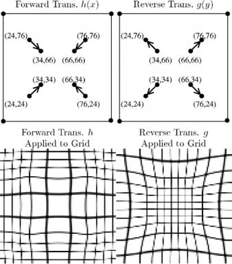
The first experiment compares the inverse consistency error associated with the traditional unidirectional landmark thin-plate spline (UL-TPS) algorithm to that of the consistent landmark thin-plate spline (CL-TPS) algorithm. This simple experiment is designed to show that the UL-TPS algorithm can have significant inverse consistency error while this error is minimized using the CL-TPS algorithm. The experiment shown in Fig. 6.4 consisted of matching eight landmarks in one image to their corresponding landmarks in a second image using both
Figure 6.4: The location of local displacements at the landmarks points for the forward, and reverse transformations of images with 100 × 100 pixels. Application of the thin-plate spline deformation fields to uniformly spaced grids for the forward and reverse transformations.

238 |
Christensen |
the UL-TPS and the CL-TPS algorithm. The arrows in the first and second panels show the displacement between the corresponding landmarks in the forward and reverse directions, respectively. The four landmarks in the corners of the images were fixed. The forward transformation h maps the four inner points to the four outer points and the reverse transformation g maps the outer points to the inner points. Applying the CL-TPS transformations to a rectangular grid shows that the forward transformation—defined with respect to a Eulerian frame of reference—causes the center of the image to expand (third panel of Fig. 6.4) while the reverse transformation causes a contraction of the central portion of the image (fourth panel of Fig. 6.4).
The top row of Fig. 6.5 shows the spatial locations and magnitudes of the inverse consistency errors of the forward and reverse transformations generated by the UL-TPS algorithm. The images in the left column were computed by taking the Euclidean norm of the difference between the forward transformation h and the inverse of the reverse transformation g−1. The images in the center column were computed in a similar fashion with g and h−1. The CL-TPS result
Figure 6.5: The left and center panels show the inverse consistency errors of the forward and reverse transformations, respectively. The tables in the right columns list the landmark errors associated with selected image points. The top and bottom rows are the inverse consistency errors associated with the unidirectional (UL-TPS) and consistent (CL-TPS) landmark thin-plate spline algorithms, respectively.