

Network Plus 2005 In Depth
.pdf72 |
Chapter 3 TRANSMISSION BASICS AND NETWORKING MEDIA |
with which data can travel over a network. In some cases—for example, telephone service over the Internet—full-duplex data networks are a requirement.
Many network devices, such as modems and NICs, allow you to specify whether the device should use halfor full-duplex communication. It’s important to know what type of transmission a network supports before installing network devices on that network. If you configure a computer’s NIC to use full-duplex while the rest of the network is using half-duplex, for example, that computer will not be able to communicate on the network.
Multiplexing
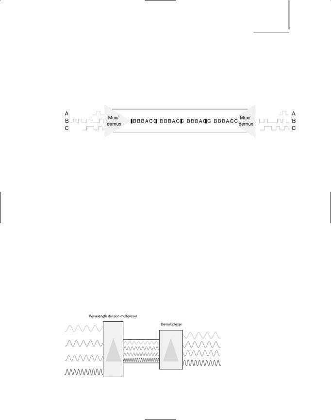
A form of transmission that allows multiple signals to travel simultaneously over one medium is known as multiplexing. To carry multiple signals, the medium’s channel is logically separated into multiple smaller channels, or subchannels. Many different types of multiplexing are available and the type used in any given situation depends on what the media, transmission, and reception equipment can handle. For each type of multiplexing, a device that can combine many signals on a channel, a multiplexer (mux), is required at the sending end of the channel. At the receiving end, a demultiplexer (demux) separates the combined signals and regenerates them in their original form.
Multiplexing is commonly used on networks to increase the amount of data that can be transmitted in a given time span. One type of multiplexing, TDM (time division multiplexing), divides a channel into multiple intervals of time, or time slots. It then assigns a separate time slot to every node on the network and, in that time slot, carries data from that node. For example, if five stations are connected to a network over one wire, five different time slots are established in the communications channel. Workstation A may be assigned time slot 1, workstation B time slot 2, workstation C time slot 3, and so on. Time slots are reserved for their designated nodes regardless of whether the node has data to transmit. If a node does not have data to send, nothing is sent during its time slot. This arrangement can be inefficient if some nodes on the network rarely send data. Figure 3-7 shows a simple TDM model.
Statistical multiplexing is similar to time division multiplexing, but rather than assigning a separate slot to each node in succession, the transmitter assigns slots to nodes according to priority and need. This method is more efficient than TDM, because in statistical multiplexing
FIGURE 3-7 Time division multiplexing
TRANSMISSION BASICS |
Chapter 3 |
73 |
time slots are unlikely to remain empty. To begin with, in statistical multiplexing, as in TDM, each node is assigned one time slot. However, if a node doesn’t use its time slot, statistical multiplexing devices recognize that and assign its slot to another node that needs to send data. The contention for slots may be arbitrated according to use or priority or even more sophisticated factors, depending on the network. Most importantly, statistical multiplexing maximizes available bandwidth on a network. Figure 3-8 depicts a simple statistical multiplexing system.
FIGURE 3-8 Statistical multiplexing
WDM (wavelength division multiplexing) is a technology used with fiber-optic cable. In fiber-optic transmission, data is represented as pulses of light, rather than pulses of electric current. WDM enables one fiber-optic connection to carry multiple light signals simultaneously. Using WDM, a single fiber can transmit as many as 20 million telephone conversations at one time. WDM can work over any type of fiber-optic cable.
In the first step of WDM, a beam of light is divided into up to 40 different carrier waves, each with a different wavelength (and therefore, a different color). Each wavelength represents a separate transmission channel capable of transmitting up to 10 Gbps. Before transmission, each carrier wave is modulated with a different data signal. Then, through a very narrow beam of light, lasers issue the separate, modulated waves to a multiplexer. The multiplexer combines all of the waves, in the same way that a prism can accept light beams of different wavelengths and concentrate them into a single beam of white light. Next, another laser issues this multiplexed beam to a strand of fiber within a fiber-optic cable. The fiber carries the multiplexed signals to a receiver, which is connected to a demultiplexer. The demultiplexer acts as a prism to separate the combined signals according to their different wavelengths (or colors). Then, the separate waves are sent to their destinations on the network. If the signal risks losing strength between the multiplexer and demultiplexer, an amplifier might be used to boost it. Figure 3-9 illustrates WDM transmission.
FIGURE 3-9 Wavelength division multiplexing

74 |
Chapter 3 TRANSMISSION BASICS AND NETWORKING MEDIA |
The form of WDM used on most modern fiber-optic networks is DWDM (dense wave division multiplexing). In DWDM, a single fiber in a fiber-optic cable can carry between 80 and 160 channels. It achieves this increased capacity because it uses more wavelengths for signaling. In other words, there is less separation between the usable carrier waves in DWDM than there is in the original form of WDM. Because of its extraordinary capacity, DWDM is typically used on high-bandwidth or long-distance WAN links, such as the connection between a large ISP and its (even larger) network service provider.
Relationships Between Nodes
So far you have learned about two important characteristics of data transmission: the type of signaling (analog or digital) and the direction in which the signal travels (simplex, half-duplex, full-duplex, or multiplex). Another important characteristic is the number of senders and receivers, as well as the relationship between them. In general, data communications may involve a single transmitter with one or more receivers, or multiple transmitters with one or more receivers. The remainder of this section introduces the most common relationships between transmitters and receivers.
When a data transmission involves only one transmitter and one receiver, it is considered a point-to-point transmission. An office building in Dallas exchanging data with another office in St. Louis over a WAN connection is an example of point-to-point transmission. In this case, the sender only transmits data that is intended to be used by a specific receiver. By contrast, broadcast transmission involves one transmitter and multiple receivers. For example, a TV station indiscriminately transmitting a signal from its tower to thousands of homes with TV antennas uses broadcast transmission. A broadcast transmission sends data to any and all receivers, without regard for which receiver can use it. Broadcast transmissions are frequently used on networks because they are simple and quick. They are used to identify certain nodes, to send data to certain nodes (even though every node is capable of picking up the transmitted data, only the destination node will actually do it), and to send announcements to all nodes. Another example of network broadcast transmission is sending video signals to multiple viewers on a network. When used over the Web, this type of broadcast transmission is called Webcasting. Figure 3-10 contrasts point-to-point and broadcast transmissions.
Throughput and Bandwidth
The data transmission characteristic most frequently discussed and analyzed by networking professionals is throughput. Throughput is the measure of how much data is transmitted during a given period of time. It may also be called capacity or bandwidth (though as you will learn, bandwidth is technically different from throughput). Throughput is commonly expressed as a quantity of bits transmitted per second, with prefixes used to designate different throughput amounts. For example, the prefix “kilo” combined with the word “bit” (as in “kilobit”) indicates 1000 bits per second. Rather than talking about a throughput of 1000 bits per second, you typically say the throughput was 1 kilobit per second (1 Kbps). Table 3-1 summarizes the terminology and abbreviations used when discussing different throughput amounts. As an example,

TRANSMISSION BASICS |
Chapter 3 |
75 |
FIGURE 3-10 Point-to-point versus broadcast transmission
a typical modem connecting a home PC to the Internet would probably be rated for a maximum throughput of 56.6 Kbps. A fast LAN might transport up to 10 Gbps of data. Contemporary networks commonly achieve throughputs of 10 Mbps, 100 Mbps, or 1 Gbps.
Table 3-1 Throughput measures
Quantity |
Prefix |
Complete Example |
Abbreviation |
1 bit per second |
n/a |
1 bit per second |
bps |
1000 bits per second |
kilo |
1 kilobit per second |
Kbps |
1,000,000 bits per second |
mega |
1 megabit per second |
Mbps |
1,000,000,000 bits per second |
giga |
1 gigabit per second |
Gbps |
1,000,000,000,000 bits per second |
tera |
1 terabit per second |
Tbps |
|
|
|
|
NOTE
Be careful not to confuse bits and bytes when discussing throughput. Although data storage quantities are typically expressed in multiples of bytes, data transmission quantities (in other words, throughput) are more commonly expressed in multiples of bits per second. When representing different data quantities, a small “b” represents

76 |
Chapter 3 TRANSMISSION BASICS AND NETWORKING MEDIA |
bits, while a capital “B” represents bytes. To put this into context, a modem may transmit data at 56.6 Kbps (kilobits per second); a data file may be 56 KB (kilobytes) in size. Another difference between data storage and data throughput measures is that in data storage the prefix kilo means “2 to the 10th power,” or “1024,” not “1000.”
Often, the term “bandwidth” is used interchangeably with throughput, and in fact, this may be the case on the Network+ certification exam. Bandwidth and throughput are similar concepts, but strictly speaking, bandwidth is a measure of the difference between the highest and lowest frequencies that a medium can transmit. This range of frequencies, which is expressed in Hz, is directly related to throughput. For example, if the FCC told you that you could transmit a radio signal between 870 and 880 MHz, your allotted bandwidth (literally, the width of your frequency band) would be 10 MHz.
Baseband and Broadband
Baseband is a transmission form in which (typically) digital signals are sent through direct current (DC) pulses applied to the wire. This direct current requires exclusive use of the wire’s capacity. As a result, baseband systems can transmit only one signal, or one channel, at a time. Every device on a baseband system shares the same channel. When one node is transmitting data on a baseband system, all other nodes on the network must wait for that transmission to end before they can send data. Baseband transmission supports half-duplexing, which means that computers can both send and receive information on the same length of wire. In some cases, baseband also supports full duplexing.
Ethernet is an example of a baseband system found on many LANs. In Ethernet, each device on a network can transmit over the wire—but only one device at a time. For example, if you want to save a file to the server, your NIC submits your request to use the wire; if no other device is using the wire to transmit data at that time, your workstation can go ahead. If the wire is in use, your workstation must wait and try again later. Of course, this retrying process happens so quickly that you don’t even notice the wait.
Broadband is a form of transmission in which signals are modulated as radiofrequency (RF) analog waves that use different frequency ranges. Unlike baseband, broadband technology does not encode information as digital pulses.
As you may know, broadband transmission is used to bring cable TV to your home. Your cable TV connection can carry at least 25 times as much data as a typical baseband system (like Ethernet) carries, including many different broadcast frequencies on different channels. In traditional broadband systems, signals travel in only one direction—toward the user. To allow users to send data as well, cable systems allot a separate channel space for the user’s transmission and use amplifiers that can separate data the user issues from data the network transmits. Broadband transmission is generally more expensive than baseband transmission because of the extra hardware involved. On the other hand, broadband systems can span longer distances than baseband.

|
TRANSMISSION BASICS |
Chapter 3 |
|
|
77 |
|
|
||||
|
|
|
|
|
|
|
In the field of networking, some terms have more than one meaning, depending on their con- |
|
|||
|
text. “Broadband” is one of those terms. The “broadband” described in this chapter is the |
|
|||
|
transmission system that carries RF signals across multiple channels on a coaxial cable, as used |
|
|||
|
by cable TV. This definition was the original meaning of broadband. However, broadband has |
|
|||
|
evolved to mean any of several different network types that use digital signaling to transmit |
|
|||
|
data at very high transmission rates. |
|
|
|
|
|
Transmission Flaws |
|
|
|
|
|
Both analog and digital signals are susceptible to degradation between the time they are issued |
|
|||
NET+ |
|
||||
|
|
|
|
|
|
4.8by a transmitter and the time they are received. One of the most common transmission flaws affecting data signals is noise.
Noise
As you learned earlier, noise is any undesirable influence that may degrade or distort a signal. Many different types of noise may affect transmission. A common source of noise is EMI (electromagnetic interference), or waves that emanate from electrical devices or cables carrying electricity. Motors, power lines, televisions, copiers, fluorescent lights, manufacturing machinery, and other sources of electrical activity (including a severe thunderstorm) can cause EMI. One type of EMI is RFI (radiofrequency interference), or electromagnetic interference caused by radiowaves. (Often, you’ll see EMI referred to as EMI/RFI.) Strong broadcast signals from radio or TV towers can generate RFI. When EMI noise affects analog signals, this distortion can result in the incorrect transmission of data, just as if static prevented you from hearing a radio station broadcast. However, this type of noise affects digital signals much less. Because digital signals do not depend on subtle amplitude or frequency differences to communicate information, they are more apt to be readable despite distortions caused by EMI noise.
Another form of noise that hinders data transmission is crosstalk. Crosstalk occurs when a signal traveling on one wire or cable infringes on the signal traveling over an adjacent wire or cable. If you have ever been on the phone and heard the conversation on your second line in the background, you have heard the effects of crosstalk. In this example, the current carrying a signal on the second line’s wire imposes itself on the wire carrying your line’s signal, as shown in Figure 3-11. The resulting noise, or crosstalk, is equal to a portion of the second line’s signal. Crosstalk in the form of overlapping phone conversations is bothersome, but does not usually prevent you from hearing your own line’s conversation. In data networks, however, crosstalk can be extreme enough to prevent the accurate delivery of data.
In addition to EMI and crosstalk, less obvious environmental influences, including heat, can also cause noise. In every signal, a certain amount of noise is unavoidable. However, engineers have designed a number of ways to limit the potential for noise to degrade a signal. One way is simply to ensure that the strength of the signal exceeds the strength of the noise. Proper cable design and installation are also critical for protecting against noise’s effects. Note that all forms of noise are measured in decibels (dB).

78 |
Chapter 3 TRANSMISSION BASICS AND NETWORKING MEDIA |
NET+ |
Cable |
4.8 |
|
|
Wire transmitting |
|
signal |
|
Wires affected |
|
by crosstalk |
|
Crosstalk |
FIGURE 3-11 Crosstalk between wires in a cable
Attenuation
Another transmission flaw is attenuation, or the loss of a signal’s strength as it travels away from its source. To compensate for attenuation, both analog and digital signals are strengthened en route so they can travel farther. However, the technology used to strengthen an analog signal is different from that used to strengthen a digital signal. Analog signals pass through an amplifier, an electronic device that increases the voltage, or strength, of the signals. When an analog signal is amplified, the noise that it has accumulated is also amplified. This indiscriminate amplification causes the analog signal to worsen progressively. After multiple amplifications, an analog signal may become difficult to decipher. Figure 3-12 shows an analog signal distorted by noise and then amplified once.
FIGURE 3-12 An analog signal distorted by noise and then amplified
TRANSMISSION BASICS |
Chapter 3 |
79 |
NET+ |
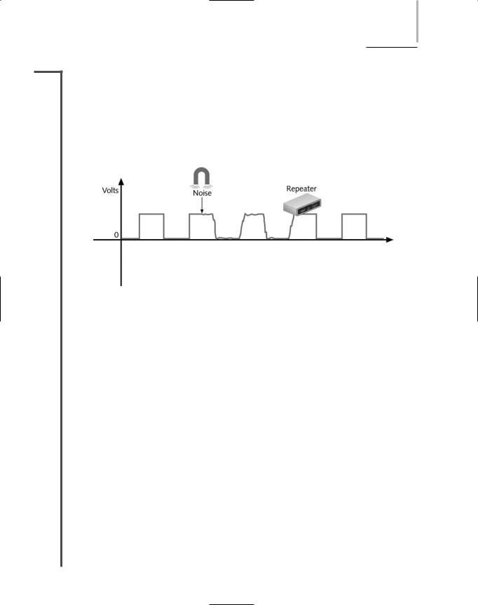
When digital signals are repeated, they are actually retransmitted in their original form, with- |
4.8out the noise they may have accumulated previously. This process is known as regeneration. A device that regenerates a digital signal is called a repeater. Figure 3-13 shows a digital signal distorted by noise and then regenerated by a repeater.
Amplifiers and repeaters belong to the Physical layer of the OSI Model. Both are used to extend the length of a network. Because most networks are digital, however, they typically use repeaters.
FIGURE 3-13 A digital signal distorted by noise and then repeated
Latency
In an ideal world, networks could transmit data instantaneously between sender and receiver, no matter how great the distance between the two. However, in the real world every network is subjected to a delay between the transmission of a signal and its eventual receipt. For example, when you press a key on your computer to save a file to the network, the file’s data must travel through your NIC, the network wire, a one or more connectivity devices, more cabling, and the server’s NIC before it lands on the server’s hard disk. Although electrons travel rapidly, they still have to travel, and a brief delay takes place between the moment you press the key and the moment the server accepts the data. This delay is called latency.
The length of the cable involved affects latency, as does the existence of any intervening connectivity device, such as a router. Different devices affect latency to different degrees. For example, modems, which must modulate both incoming and outgoing signals, increase a connection’s latency far more than hubs, which simply repeat a signal. The most common way to measure latency on data networks is by calculating a packet’s RTT (round trip time), or the length of time it takes for a packet to go from sender to receiver, then back from receiver to sender. RTT is usually measured in milliseconds.
Latency causes problems only when a receiving node is expecting some type of communication, such as the rest of a data stream it has begun to accept. If that node does not receive the rest of the data stream within a given time period, it assumes that no more data is coming. This assumption may cause transmission errors on a network. When you connect multiple

80 |
|
|
Chapter 3 TRANSMISSION BASICS AND NETWORKING MEDIA |
|
|
||||
|
|
|
|
|
|
|
network segments and thereby increase the distance between sender and receiver, you increase |
||
NET+ |
|
|
||
4.8the latency in the network. To constrain the latency and avoid its associated errors, each type of cabling is rated for a maximum number of connected network segments and each transmission method is assigned a maximum segment length.
Common Media Characteristics
Now that you are familiar with variations in data signaling, you are ready to learn more about the physical and atmospheric paths that these signals traverse. When deciding which kind of transmission media to use, you must match your networking needs with the characteristics of the media. This section describes the characteristics of all types of media, including throughput, cost, size and scalability, connectors, and noise immunity.
Throughput
Perhaps the most significant factor in choosing a transmission method is its throughput. All media are limited by the laws of physics that prevent signals from traveling faster than the speed of light. Beyond that, throughput is limited by the signaling and multiplexing techniques used in a given transmission method. Transmission methods using fiber-optic cables achieve faster throughput than those using copper or wireless connections. Noise and devices connected to the transmission medium can further limit throughput. A noisy circuit spends more time compensating for the noise and, therefore, has fewer resources available for transmitting data.
Cost
The precise costs of using a particular type of cable or wireless connection are often difficult to pinpoint. For example, although a vendor might quote you the cost-per-foot for new network cabling, you might also have to upgrade some hardware on your network to use that type of cabling. Thus, the cost of upgrading your media would actually include more than the cost of the cabling itself. Not only do media costs depend on the hardware that already exists in a network, but they also depend on the size of your network and the cost of labor in your area (unless you plan to install the cable yourself ). The following variables can all influence the final cost of implementing a certain type of media:
Cost of installation—Can you install the media yourself, or must you hire contractors to do it? Will you need to move walls or build new conduits or closets? Will you need to lease lines from a service provider?
Cost of new infrastructure versus reusing existing infrastructure—Can you use existing wiring? In some cases, for example, installing all new Category 7 UTP wiring may not pay off if you can use existing Category 5 UTP wiring. If you replace only part of your infrastructure, will it be easily integrated with the existing media?

COMMON MEDIA CHARACTERISTICS |
Chapter 3 81 |
Cost of maintenance and support—Reuse of an existing cabling infrastructure does not save any money if it is in constant need of repair or enhancement. Also, if you use an unfamiliar media type, it may cost more to hire a technician to service it. Will you be able to service the media yourself, or must you hire contractors to service it?
Cost of a lower transmission rate affecting productivity—If you save money by reusing existing slower lines, are you incurring costs by reducing productivity? In other words, are you making staff wait longer to save and print reports or exchange e-mail?
Cost of obsolescence—Are you choosing media that may become passing fads, requiring rapid replacement? Will you be able to find reasonably priced connectivity hardware that will be compatible with your chosen media for years to come?
Size and Scalability
Three specifications determine the size and scalability of networking media: maximum nodes per segment, maximum segment length, and maximum network length. In cabling, each of these specifications is based on the physical characteristics of the wire and the electrical characteristics of data transmission. The maximum number of nodes per segment depends on attenuation and latency. Each device added to a network segment causes a slight increase in the signal’s attenuation and latency. To ensure a clear, strong, and timely signal, you must limit the number of nodes on a segment.
The maximum segment length depends on attenuation and latency plus the segment type. A network can include two types of segments: populated and unpopulated. A populated segment is a part of a network that contains end nodes. For example, a hub connecting users in a classroom is part of a populated segment. An unpopulated segment, also known as a link segment, is a part of the network that does not contain end nodes, but simply connects two networking devices such as hubs.
Segment lengths are limited because after a certain distance, a signal loses so much strength that it cannot be accurately interpreted. The maximum distance a signal can travel and still be interpreted accurately is equal to a segment’s maximum length. Beyond this length, data loss is apt to occur. As with the maximum number of nodes per segment, maximum segment length varies between different cabling types. The same principle of data loss applies to maximum network length, which is the sum of the network’s segment lengths.
Connectors and Media Converters
NET+ |
Connectors are the pieces of hardware that connect the wire to the network device, be it a file |
1.4server, workstation, switch, or printer. Every networking medium requires a specific kind of connector. The type of connectors you use will affect the cost of installing and maintaining the network, the ease of adding new segments or nodes to the network, and the technical expertise required to maintain the network. The connectors you are most likely to encounter on modern networks are illustrated throughout this chapter and shown together in Appendix C.