Мақолалар

The Importance of Risk Assessment in the Context of Investment Project Management: A Case Study

Author(s):

M. Bernadete Junkesa (а), Anabela P. Teresob (b), Paulo S.L.P. Afonsob (b)

(a) Departamento de Ciências Contábeis, Fundação Universidade Federal de Rondônia, Campus Cacoal, Rondônia, Brasil

(b) Centro Algoritmi, Escola de Engenharia, Universidade do Minho, Campus de Azurém, 4800-058, Guimarães, Portugal

Conference on ENTERprise Information Systems / International Conference on Project MANagement / Conference on Health and Social Care Information Systems and Technologies, CENTERIS / ProjMAN / HCist 2015 October 7-9, 2015

Available online at www.sciencedirect.com//

Procedia Computer Science 64 ( 2015 ) 902 – 910

Abstract

Abstract Risk management is an important component of project management. Nevertheless, such process begins with risk assessment and evaluation. In this research project, a detailed analysis of the methodologies used to treat risks in investment projects adopted by the Banco da Amazonia S.A. was made. Investment projects submitted to the FNO (Constitutional Fund for Financing the North) during 2011 and 2012 were considered for that purpose. It was found that the evaluators of this credit institution use multiple indicators for risk assessment which assume a central role in terms of decision-making and contribute for the approval or the rejection of the submitted projects; namely, the proven ability to pay, the financial records of project promotors, several financial restrictions, level of equity, level of financial indebtedness, evidence of the existence of a consumer market, the proven experience of the partners/owners in the business, environmental aspects, etc. Furthermore, the bank has technological systems to support the risk assessment process, an internal communication system and a unique system for the management of operational risk.

Introduction

Risk is, fundamentally, the possibility of financial loss. It is used as a synonym of uncertainty and refers to the variability of returns associated with an investment project1 . As the projects may be independent or mutually exclusive, it is crucial the use of analytical techniques in accordance with each specific situation. The existence of uncertainty means that decisions and behaviors are not based on routines. Indeed, financial decisions are taken in environments of uncertainty. Thus, the measurement and management of risks are becoming increasingly important. Decisions taken at the present time have their results conditioned by future events and may influence the later thus they may result in potential gains or losses2 . Considering these facts, it can be seen that, for the purpose of this analysis, the project evaluator or decision maker can find a diversity of problems, making unfeasible the use of a single mechanical process for the assessment of their viability3 . In this sense, banks cannot always check if the projects that will be financed will be profitable or not, as well as the degree of risk of financing them. Small businesses are particularly vulnerable and dependent on financial institutions that offer credit because they have not access to capital markets. This situation causes that small businesses have less credit options being subject to financial imbalances and higher levels of financial dependency than bigger companies4 . Furthermore, small companies are less prepared for risk assessement and project evaluation, and this situation augments their level of financial dependency. Considering these facts, a case study was conducted in a public institution of credit named Banco da Amazonia S.A., located in the Amazon region. In Brazil, the investors and the bodies in charge for fiscal and financial incentives have been demanding specialized professionals, with good skills in the preparation and analysis of investment projects, in order to ensure the quality of the evaluations. In this context, the introduction of risk evaluation as an important process in the analysis of investments of commercial and industrial projects is absolutely necessary5 . Thus, in this research project, a detailed analysis of the methodologies used to treat risks in investment projects adopted by the Banco da Amazonia S.A., located in the Amazon Region, Brazil, was made. It was considered the portfolio of investment projects in the years of 2011 and 2012 of the FNO (Constitutional Fund for Financing the North). This fund supports the development of the northern region of the country, located in the Amazon Region, Brazil. Project and risk evaluation are important initial steps that may contribute to future project management success. A poor quality risk assessment process may compromises the project and will turn risk management more demanding. In this context, not only which metrics but also how and why the process is conducted are important. The case study offers interesting insights and may contribute to understand the role and the relationship of risk assessment and risk management in the context of project management.

Assessment and management of risks in investment projects

A risk event can be considered as a discrete occurrence that affects a project for the better or for the worse, while uncertainty occurs when there is no sufficient and clear information available to decision makers, reducing confidence on evaluating alternatives and their risks, thus, complicating decision-making. Uncertainty is defined as the lack of objective probability distributions associated with the events that may occur6 . In this context it can be presented in three generic groups7 : uncertainty about the prices and components of investment, uncertainties regarding the deadlines for implementing the schedule and uncertainties regarding the occurrence of events. Furthermore, risk, in its basic sense, is the possibility of financial loss or, more formally, the variability of returns associated with a particular asset8 . Decision-making based on risk (Risk-Based Decision Making - RBDM) is essential for an effective and efficient management of projects9 . Risks10,11,12 can be divided into 10 categories: 1) Resources related risks; 2) Technical risks; 3) Business risks; 4) Programming risks; 5) Economic risks; 6) Priorise risks;7) Enterprise risks; 8) Financial risks; 9) Country risks; 10) Environmental risks. The process of risk assessment in investment projects can be defined as being composed of five steps13,14:estimate the expected future cash flows for the project, determine the discount rate (opportunity cost of capital) to discount the expected future cash flows, calculate the financial indicators, mainly the Net Present Value (NPV) of expected future cash flows, set the cost of the project and compare it with the NPV of the cash flows of the project and make the decision to invest or not in the project. Furthermore, the process of risk evaluation of an investment project is typically made through a sensitivity and risk analysis. Typically, in the sensitivity and risk analysis, it is possible to measure the impact on financial indicators, such as the NPV and the Internal Rate of Return (IRR), when a certain relevant parameter of investment varies. It is then possible to determine the value of each estimated parameter that redefines the NPV of the project, allowing the acceptance or rejection of the project15,16,17. The Break-even point of an investment project is the level of production and sales for which the project produces neither profits nor losses18. The Break-even Analysis is a relatively simple method but it is important and should be used for the initial analysis of an investment project in a context of uncertainty19. The risk analysis examines various possible scenarios, where a given combination of factors is considered. Typically, the procedure of scenario analysis considers three types of scenarios for the risk analysis of the project: Most Likely, Optimistic and Pessimistic. The first scenario is considered, by specialists in business projects, the one that uses the expected value or the more "representative" value for each of the estimates of the project. In the optimistic scenario, certain parameters of interest on the part of the base scenario are increased in value, while the opposite occurs in the pessimistic scenario, where the values decrease with respect to the base scenario20. In the risk analysis it is assumed that the uncertainties associated with the estimates of the parameters are regarded as somewhat subjective. Thus, a more efficient approach consists in the construction of random scenarios, however probable, from the distributions of probabilities of the variables of competing interests21. The Monte Carlo method is a sampling technique employed to operate numerically complex systems that have random components22. Probability analysis uses Monte Carlo simulation to model the combined effect of numerous risk factors according to their relative frequencies. A possible problem is determining the probability distributions of the different variables, especially in some industries where these distributions are not available, as each project is unique and affected by different risk factors. Another limitation of using probability analysis is that the influence of non-monetary (qualitative) aspects on projects is often not easily quantified23. Furthermore, with the increasing popularity of privately financed and operated projects, a systematic evaluation of investment options may be needed, especially if they are competing for the same capital resource. The value of each parameter is affected by a myriad of risks and uncertainties which are often difficult to quantify. In addition, these techniques do not allow for the non-monetary (qualitative) factors to be considered in assessing the investment option. To ignore these aspects can cause the failure of a project despite favorable financial components24. One way to overcome the above shortcomings is to use the Possibility Theory where the user needs only to determine a possible range, and perhaps even a most likely value for each investment parameter, without the input of each factor's relative frequency23. The possibility theory is based on the concept that all values within a certain range are possible, with the exact value being unknown. Using this assumption, the authors23,24 developed a system for the integration of monetary and non-monetary factors in investment appraisal, using the Possibility Theory to represent the possible values of each parameter that may affect the overall preference for a particular project. They used the NPV as the monetary evaluation function, combining all possible factors affecting the NPV, and obtaining its monetary distribution. For the non-monetary factors, they also used possibility distributions and define a nonmonetary possibility distribution using weights for each factor. Finally, they calculated the overall project ranking using the ranking index method. Some authors argue that, for the analysis and evaluation of investment projects, such techniques are better suited to cope with operation flexibility and other strategic aspects than traditional capital budgeting methods or discounted cash flow approaches, like NPV25. These critiques have led to the emergence of real options analysis (ROA) for valuing managerial flexibility in projects.

The contingent claims analysis approach to ROA uses market-priced securities to construct a portfolio that replicates the payoffs of the project and determines the project value using a no-arbitrage argument. The risk-neutral probability approach is an equivalent method that computes adjusted probabilities that allow valuing the project using risk-free discount rates. Both methods use geometric Brownian motion processes or binomial trees to model the project’s uncertainty26. The decision analysis can be used for projects that involve sequential decisions. This means, that in many cases, there is not simply a single decision, but several sequential decisions. Thus “blind” acceptance of projects is not necessary, where only the decisions of acceptance or rejection of the project are considered, ignoring the decisions for subsequent investments that can be made17.

Methodology

In this research project, a previous characterization of the Banco da Amazonia S.A. was made, regarding the analysis of the process of approval of investment projects in 2011 and 2012 of the FNO program. Furthermore, the data was obtained following a specific case study protocol. Most of the information was obtained by means of interviews and questionnaires, prepared by the researchers in three different stages. In a first moment it was conducted an interview with the superintendent responsible for the release of financial resources. In the second phase, a questionnaire was designed and applied to collect information on the characterization of the proponent of the investment project, objectives of the funding, description of the requested amount, types of guarantees and forms of payment of financing among others. The third and last phase was used to understand the process of risk assessment and to study the indices and indicators used by the bank in the risk analysis of investment projects. Due to the fact that the projects have basically the same pattern of development, the researchers have chosen to observe 20 approved projects, 10 in the year of 2011 and the other 10 in the year of 2012.

Case Study

The Banco da Amazonia was created in 1942 with the name of Banco de Crédito da Borracha (i.e. Rubber Credit Bank). Its objectives were to promote the development of incentives for the exploitation of natural rubber, in support of the Allied Forces during the Second World War. In 1950, the bank has been transformed into the Banco de Crédito da Amazónia (BCA) and began to participate in a more comprehensive form in the process of regional development, financing all economic segments of the Region. From 1966, it acts as the Financial Agent of the credit policy of the Federal Government for the Amazon Region, assuming the name of Banco da Amazonia27. Through its Environmental Policy, the Banco da Amazonia seeks to incorporate the components of economic, environmental, and social sustainability in the whole spectrum of its activities, aiming to promote the solidification of local innovative productive systems, inserted in projects aligned to the assumptions of sustainable development and articulated to domestic and international markets28. Aligned with the Principles of the Basel Accord and the regulations of the Central Bank of Brazil, the risk management of the Banco da Amazonia permeates all units who manage processes/risks, and has the objective to manage the risks in all the activities of the company, in order to maximize the opportunities and minimize the negative effects. The Banco da Amazonia considers risk assessment fundamental for the decision-making process, because it provides greater stability, better capital allocation and optimization of the risk versus return. In compliance with legal and regulatory requirements and before the stage of maturity of processes and systems available, the Bank has implemented a risk management framework that enables the handling of legal requirements, in accordance with the standardized, simplified and basic methods. As a technological support to risk management, the Bank has in its structure an internal communication system based on the disclosure of standards for their employees through the intranet and a unique system for the management of operational risk. The management of the credit risk includes the monitoring of the Probability of Default (PD), the Loss Given Default (LGD), Provision for Credit Losses (PCL) and calculation of RWAcpad (plot relative to the exposure to credit risk). In addition to the system that supports the Management of Market Risk and Liquidity, to the management and monitoring of exposures to these risks.In accordance with its internal guidelines, the Banco da Amazonia invests in the continuous improvement of the processes and practices of risk management, in line with the benchmarks of international market and with the New Basel Accord, known as Basel II, and the adjustments promoted by Basel III²⁹.

Analysis and Discussion

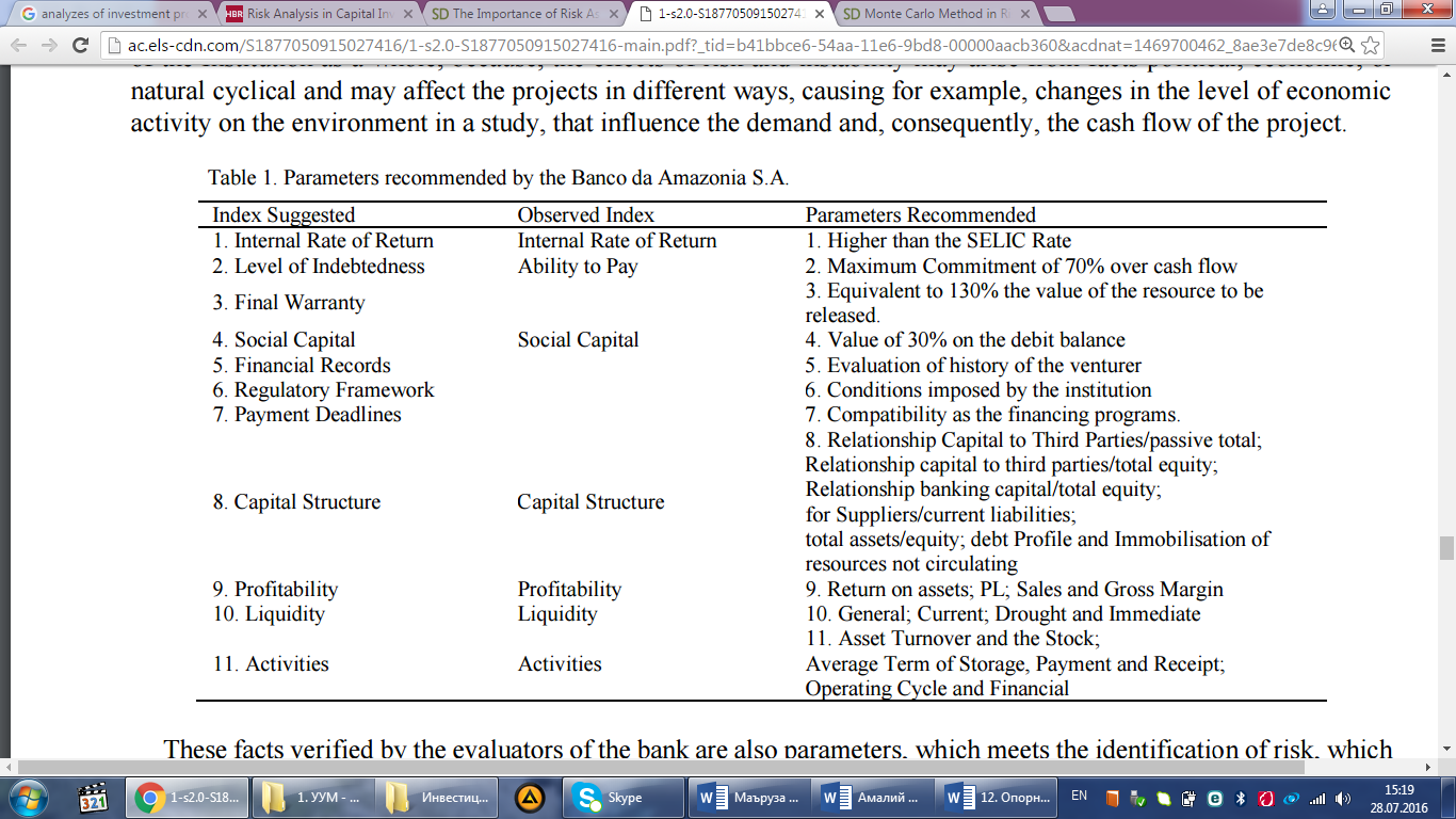
The decision-making process for the approval of a project by the Banco da Amazonia S.A. has the following parameters: the ability-to-pay in proven cash flow projected investment; the financial records and restrictions, level of equity; the financial indebtedness; existence of a consumer market; experience of members/owners in the industry in which they will operate; credit history check with the Banco da Amazonia S.A., environmental aspects required; and the ability to integrate with other local actors. These factors are related to the lack of sufficient information or uncertainty6 . In the risk analysis, the credibility of the project is analysed, which begins by evaluating the past of the entrepreneurs, the analysis of historical results extracted from the accounts of the company and/or affiliates, etc.7 On the other hand, when the bank receives proposals that may have some possibility of risk, they are returned to the client to reformulate the project in order to minimize the risk, and even so there may still subsist risk that should be considered in the project, deciding who will assume it (the client, the bank or other element). This type of situation is in line with the literature9,30, in which the basis for decision-making is provided by project risk evaluation, which takes into account the possibilities of any risks or uncertainties related with the project. In this sense9 , in decisionmaking process based on risk, it is vital to ensure a complete and accurate risk evaluation30. From 2013 onwards the Banco da Amazonia S.A., necessarily presents information about the indicators that are required by the Central Bank of Brazil (BACEN), in response to Circular no. 3,678 /13, which implies for the disclosure of information relating to risk management, the determination of the amount of assets weighted by risk (RWA or Risk Weighted Assets) and the determination of the Reference Assets (RA), aligned to good banking practice in relation to the new rules of capital and in accordance with the norms of the Institution. In the analysis of investment projects, due to the fact that financial institutions are dependent on borrowed capital, it was observed that the credit institution analysts use instruments of accounting to check how much the institution used capital to third parties in relation to its own capital available for lending. As far as the viability indices demonstrated, the evaluators measure the capacity of profitability on the capital invested by the institution itself in projects and other types of financial transactions. On the other hand, the indices of liquidity indicate the capacity to honor the commitments and payments of obligations of the institution. The index of activities refers the revolutions suffered by capital in the sense of how many times the financial resources were employed, how they were recovered, how long it took to recover the investment. It is an operating cycle that reflects the operational reality of the institution. Investors have several methods for the analysis of investments9,36,37 . Nevertheless, according to the information obtained from the superintendent of the Banco da Amazonia S.A., the evaluators should give particular attention to the indicators related to profitability and liquidity. From the case study, it was possible to realize that the parameters identified in the analysis of the project fall under 10 types of categories10,11,12, which may be included in 5 different steps for the evaluation procedure14,31. It was also found that the Banco da Amazonia S.A. follows the levels of risk of a project, explained in the Resolution 2682/1999 of the National Monetary Council - CMN/BACEN† , which deals with delays on the liquidity, ranging from AA (low risk), A, B, C, D, E, F, G, to H (high risk). Within these parameters, the Banco da Amazonia S. A., only operates with customers between "AA and C". In this sense, some authors argue that for the analysis and evaluation of investment projects, real option are more suitable for dealing with the flexibility of strategic aspects than traditional methods25,32 . The approach of risk-neutral probabilities is an equivalent method that computes adjusted odds that let you enhance the project using discount rates free of risk. Both methods use processes of Brownian motion or geometric binomial trees to model the uncertainty of the project26. These irregularities in many situations can be framed in the analysis of sensitivity and risk, verifying the impact on financial indicators, allowing to accept or reject the project15, 16,17,19. In this research it was found that the decision-makers of the Banco da Amazonia S.A. make the diagnosis of risks of the viability of financing of a project, based on the analysis of consumer market, existing data on industry, sector organizations and research institutes, as well as by indicators such as Pay-Back, NPV, IRR and discounted cash flow, in terms of sensitivity analysis exchange data of costs or revenues provided, as described in the literature23,24. Regarding the warranties, regularities considered inconsistent by the analysis team might leave room for suspicion that the values where overestimated and there was no definition of the criteria used in its calculations, creating the need for reassessment, with additional expenses and deterioration of the relationship with the client. In the attachments that come with the projects, often occurs lack of several documents like: constituent documents and financial statements of affiliated and/or controlled companies; lease with a term smaller than the requested by the funding and without renewal clause; lack of copies of contractual instruments of the debts listed in the SCR (credit IS); lack of documentation about machinery, equipment or vehicles to be purchased. After the registration analysis of the project leader and regulatory framework, a market analysis is made for the evaluation of the acceptance of the projected sales, the assessment of the adequacy of the structure of revenues and costs, projected investments, working capital needs, uses and sources and ability to pay and cash flow. Information Systems (IS) are also checked, such as: records SERASA (centralised bank service), SCR, Central Bank IS, Ministry of Labor IS, among others, as well as the system of risk assessment and management. The internal statistics for the evaluation of default rate and performance by activity, region and size are also analysed. The proposed investment projects submitted to the Banco da Amazonia S.A. are mostly private projects. This is a result of the policy of the FNO administration, whose goal is to contribute to the promotion of economic and social development of the region through funding productive sectors. In this study, the projects are mainly related to the productive activity, in need of investments in fixed assets (replacement, expansion, modernisation, innovation and social investments)31. The Banco da Amazonia S.A., is influenced by economic occurrences at international level, the political stability exerts great influence on issues such as inflation, interest rates and international image, which also have an impact in a different way on the investment projects33. This can be observed when the bank in 2011 and 2012 had a reduction in the cost of acquisition of resources due to economic policy of the country, which is reflected in lower rates paid by credit borrowers. If there are irregularities, these can be cumbersome to operate with the company, which is one of the strategies of risk management, because the bank has to be careful to run the lowest possible risk34. After the feasibility of the project is defined, which concerns the planning and management of long-term expenses investment and fund-raising, the risk analysis of the project is done, whose parameters also indicate its viability or not35. From the cash flow, indicators such as IRR and NPV are extracted. Some studies mention that sensitivity analysis allows to separate the ranges of acceptance or rejection of the project15,16,17. This diversification forces the evaluators of the bank to have specific strategies for each case under analysis. For this reason, in the literature3 , for project analysis, the evaluator or decision maker may find a diversity of problems, which makes it impossible to use a single mechanical process for viability assessment. In this process of evaluation of investment projects made by the bank, it also has been found that the steps followed are: project identification; definition of objectives; ability to pay; technical, economic and financial aspects; productive process; income; economic-financial indicators and others, that fall under the five stages of evaluation process of a project13,14. Even in this analysis, it has been identified that the bank uses tools of engineering economics in investment decisions by choosing alternatives supported by technical, economic or financial decision making, when there is the ability to pay36,37,38. In general terms, it was observed that the evaluators, following the parameters recommended by the Banco da Amazonia S.A., analyse the IRR, the Ability to Pay, etc. Table 1 presents the parameters recommended by the Banco da Amazonia S.A. grouped into indexes (observed in the database and suggested by this research). The indices suggested can increase the effectiveness of the procedures for the evaluation of risk in investment projects that capture financial resources of the FNO. For supporting new methodologies for the management of risks, since 2013 the bank has in its structure an internal communication system based on disclosure standards for its employees through the intranet; a unique system for Management of Operational Risk, which is used to record risks and incidents and feed databases of operating losses.

Another system for the Management of Credit Risk, which allows the monitoring of the probability of default (PD), the loss given default (LGD), provision for credit losses (PCL), the calculation of RWAcpad (plot relative to the exposure to credit risk), in addition to the system of Management of Market Risk and Liquidity, to the management and monitoring of exposure to these risks. For this reason, the management of credit risk in the bank permeates the whole process of granting, monitoring, billing, and credit recovery, encompassing the activities of various areas. The construction and development of an environment of risk management in investment projects, requires the participation, commitment and the involvement of the Institution as a whole, because, the effects of risk and instability may arise from facts political, economic, or natural cyclical and may affect the projects in different ways, causing for example, changes in the level of economic activity on the environment in a study, that influence the demand and, consequently, the cash flow of the project.

These facts verified by the evaluators of the bank are also parameters, which meets the identification of risk, which determines what are the risks that may affect the project and documenting the characteristics of each one, quantify these risks and are looking for alternatives to optimize the exploitation of possible results, and that define steps to optimize the exploitation of the opportunities, as well as control of the risks that may arise during the course of the project. If there are irregularities, these can be cumbersome if you operate with the company, is one of the strategies of risk management, because the bank has to be careful to run the lowest possible risk34. In relation to the projects delivered, it was found that irregularities such as project without the heading of the fortifier or without its number in the council of the category, or without the heading of responsible for company, in all its leaves; projected revenue overestimated without due justification convincing marketable; lack of consistent information on market inputs (origin, sufficiency, etc.) and products (buyers, competitors, etc.); lack of debt service on existing cash flow; deficits of deployment without information on the own resources to cover; deadlines are incompatible with the ability to pay and/or proposed activity

Conclusions

It was noticed that the bank is cautious with the approval of investment projects and uses several methods for the analysis of a project according to its levels of risk, explained in the Resolution 2682/1999 from the National Monetary Council (CMN/BACEN). Each one of these methods is focused on different variables, which can subsidize the decision making for the release of funds with the lowest possible risk, during the implementation of the project. In the evaluation of the methodologies adopted by the Banco da Amazonia S.A., based on their reports, it was found that the institution follows the principles of the Basel accord and the regulations of Central Bank of Brazil, to manage the risks involved in all activities of the institution, in order to maximize the opportunities and minimize the negative effects.

It considers the risk management fundamental to the decision-making process, which provides greater stability, better application of capital and optimization of risk versus return. Since 2013 the bank is improving the methodologies of risk management, with an internal communication system developed for the management of operational risk, to monitor the Probability of Default (PD), the Loss Given Default (LGD), the Provision for Credit Losses (PCL) and calculate the RWAcpad (plot relative to the exposure to credit risk), in addition to the system of Management of Market Risk and Liquidity, to the management and monitoring of exposures to these risks. Furthermore, it was found that the decision-maker uses several approaches to make a diagnosis of the risks of feasibility of the projects based on the analysis of the consumer market, segment entities and industry publications, the ability to pay, verified by indicators as Pay-Back, NPV, IRR, discounted cash flow, and in sensitivity analysis, by changing cost data or forecasted revenues

References

1. Powel JE. Q&A: Evaluating risk for project success. Enterprise Systems Journal 2011. 2. Bell MZ. Business continuity during a recession. Risky Thinking 2009. 3. Simić N, Vratonjić V, Berić I. Methodologies for the evaluation of public sector investment projects. Megatrend Review 2011; 8 (1): 113-129. 4. Berger AN, Udell GF. Small business credit availability and relationship lending: the importance of bank organisational structure. The Economic Journal 2002, 112(477): F32-F53. 5. Fonseca, FWF. Administração financeira e orçamentária. IESDE Brasil SA; 2009. 6. Manktelow J. Risk Analysis Risk analysis and risk management: evaluating and managing risks 2015. 7. Helliar CV, Lonie AA, Power DM, Sinclair CD. Managerial Attitudes to Risk: a comparison of Scottish chartered accountants and U.K. managers. Journal of International Accounting, Auditing & Taxation 2002, 11(2): 165-190. 8. Gitman LJ. Princípios de administração financeira. Pearson, 2010. 9. Wang J, Yuan H. Factors affecting contractors’ risk attitudes in construction projects: Case study from China. International Journal of Project Management 2011, 29: 209–219. 10. Bergamini Jr. S, Borges LFX, Motta RDR, Calôba GM, Villa-Forte LN. Modelo de Avaliação de Risco de Crédito em Projetos de Investimento quanto aos Aspectos Ambientais. IBEA Annual Congress. Puerto Vallarta - Mexico, November-20-22, 2003. 11. Jutte B. 10 Golden Rules of Project Risk Management. Project Smart 2015. 12. Jiang H., Ruan J. Investment risks assessment on high-tech projects based on analytic hierarchy process and BP neural network. Journal of networks 2010, 5(4): 393-402. 13. Finnerty JD. Project finance: engenharia financeira baseada em ativos. Rio de Janeiro: Qualitymark; 1999. 14. Samanez CP. Matemática financeira: aplicações à análise de investimentos. Makron Books; 1999. 15. Lapponi JC. Avaliação de projetos de investimento: modelos em excel. Lapponi Treinamento; 1996. 16. Saunders A, Cornett MM, McGraw PA. Financial institutions management: A risk management approach (Vol. 8). McGraw-Hill/Irwin: 2006. 17. Tereso AP. Análise de Decisão. Apostila da UC de Análise de Sistemas - Mestrado em Engenharia de Sistemas; 2010. 18. Adler, HA. Economic appraisal of transport projects: a manual with case studies. National Technical Information Service; 1987. 19. Jovanović P. Application of sensitivity analysis in investment project evaluation under uncertainty and risk. International Journal of Project Management 1999; 17(4): 217–222. 20. Kotter JP. Change management: driving Successful Change. Project Smart 2015. 21. Trapp ACG, Corrar LJ. Avaliação e gerenciamento do risco operacional no Brasil: análise de caso de uma instituição financeira de grande porte. Revista Contabilidade & Finanças 2005; 16(37): 24-36. 22. Prado D. Teoria das filas e da simulação. Belo Horizonte, MG: Editora de Desenvolvimento Gerencial, 2; 1999. 23. Mohamed S, McCowan AK. Modelling project investment decisions under uncertainty using possibility theory. International Journal of Project Management 2001; 19(4): 231–241. 24. Toakley AR. Risk analysis of project development portfolios: a review of research needs. Australian Institute of Building Papers 1997. 25. Trigeorgis L. Real options: managerial flexibility and strategy in resource allocation. The MIT Press; 1996. 26. De Reyck B, Degraeve Z, Vandenborre R. Project options valuation with net present value and decision tree analysis. European Journal of Operational Research 2008; 184(1): 341–355. 27. Banco da Amazônia. FNO - Amazônia Sustentável 2015. 28. Banco da Amazônia. Relatório de Gerenciamento de Risco 2015. 29. Banco Central do Brasil. 2015. Available at http://www.bcb.gov.br/. 30. Carey M. Determining Risk Appetite. 2015. Available at http://www.continuitycentral.com/feature0170.htm. 31. Menezes HC. Princípios da gestão financeira. 12a ed. Lisboa: Editorial presença; 2010. 32. Dixit AK, Pindyck RS. The options approach to capital investment. Real options and investment under uncertainty: Classical readings and recent contributions 2001, 61-78. 33. Damodaran A. Finanças corporativas aplicadas. Bookman; 2002. 34. Bell MZ. Does Pure Risk Exist in Business. Risky thinking, Albion Research Ltd; 2005. 35. Evangelista MLS. Estudo comparativo de análise de investimentos em projetos entre o método do VPL e o de opções reais: o caso cooperativa de crédito - Sicredi Noroeste. Master dissertation, UFSC: Florianópolis, 2006. 36. Comissão Europeia. Manual de Análise de Custos e Benefícios dos Projectos de Investimentos. 2003. 37. Watts Jr, John M, Chapman RE Engineering Economics. Section 5, Chapter 7, SFPE Handbook of Fire Protection Engineering, NFPA, Quincy MA, 2002. p.93-104. 38. Mota R, Caloba GM, Neves C, Costa RP, Nakagawa M. Engenharia economica e finanças. Campus – RJ; 2009.

Risk Analysis in Capital Investment

Risk Analysis in Capital Investment

Risk Analysis in Capital Investment

Risk Analysis in Capital Investment

Author(s):

David B. Hertz

Harvard Business Review

Available online at https://hbr.org/1979/09/risk-analysis-in-capital-investment

This article is about FINANCIAL MANAGEMENT

A version of this article appeared in the September 1979 issue of Harvard Business Review

When this article was first published, David B. Hertz was a principal with McKinsey & Company, Inc., the management consulting firm. He is currently a senior director there as well as chairman of the board of a new magazine, Prime Time. He is the author of a follow-up article in HBR entitled “Investment Policies that Pay Off” (January–February 1968) in addition to several books, including New Power for Management: Computer Systems and Management Science (McGraw-Hill, 1969) and The Theory and Practice of Industrial Research (McGraw-Hill, 1949).

Abstract

How can business executives make the best investment decisions? Is there a method of risk analysis to help managers make wise acquisitions, launch new products, modernize the plant, or avoid overcapacity? “Risk Analysis in Capital Investment” takes a look at questions such as these and says “yes”—by measuring the multitude of risks involved in each situation. Mathematical formulas that predict a single rate of return or “best estimate” are not enough. The author’s approach emphasizes the nature and processing of the data used and specific combinations of variables like cash flow, return on investment, and risk to estimate the odds for each potential outcome. Managers can examine the added information provided in this way to rate more accurately the chances of substantial gain in their ventures. The article, originally presented in 1964, continues to interest HBR readers. In a retrospective commentary, the author discusses the now routine use of risk analysis in business and government, emphasizing that the method can—and should—be used in any decision-requiring situations in our uncertain world.

Of all the decisions that business executives must make, none is more challenging—and none has received more attention—than choosing among alternative capital investment opportunities. What makes this kind of decision so demanding, of course, is not the problem of projecting return on investment under any given set of assumptions. The difficulty is in the assumptions and in their impact. Each assumption involves its own degree—often a high degree—of uncertainty; and, taken together, these combined uncertainties can multiply into a total uncertainty of critical proportions. This is where the element of risk enters, and it is in the evaluation of risk that the executive has been able to get little help from currently available tools and techniques.

There is a way to help the executive sharpen key capital investment decisions by providing him or her with a realistic measurement of the risks involved. Armed with this gauge, which evaluates the risk at each possible level of return, he or she is then in a position to measure more knowledgeably alternative courses of action against corporate objectives.

Need for New Concept

The evaluation of a capital investment project starts with the principle that the productivity of capital is measured by the rate of return we expect to receive over some future period. A dollar received next year is worth less to us than a dollar in hand today. Expenditures three years hence are less costly than expenditures of equal magnitude two years from now. For this reason we cannot calculate the rate of return realistically unless we take into account (a) when the sums involved in an investment are spent and (b) when the returns are received.

Comparing alternative investments is thus complicated by the fact that they usually differ not only in size but also in the length of time over which expenditures will have to be made and benefits returned.

These facts of investment life long ago made apparent the shortcomings of approaches that simply aver-aged expenditures and benefits, or lumped them, as in the number-of-years-to-pay-out method. These shortcomings stimulated students of decision making to explore more precise methods for determining whether one investment would leave a company better off in the long run than would another course of action.

It is not surprising, then, that much effort has been applied to the development of ways to improve our ability to discriminate among investment alternatives. The focus of all of these investigations has been to sharpen the definition of the value of capital investments to the company. The controversy and furor that once came out in the business press over the most appropriate way of calculating these values have largely been resolved in favor of the discounted cash flow method as a reasonable means of measuring the rate of return that can be expected in the future from an investment made today.

Thus we have methods which are more or less elaborate mathematical formulas for comparing the outcomes of various investments and the combinations of the variables that will affect the investments. As these techniques have progressed, the mathematics involved has become more and more precise, so that we can now calculate discounted returns to a fraction of a percent.

But sophisticated executives know that behind these precise calculations are data which are not that precise. At best, the rate-of-return information they are provided with is based on an average of different opinions with varying reliabilities and different ranges of probability. When the expected returns on two investments are close, executives are likely to be influenced by intangibles—a precarious pursuit at best. Even when the figures for two investments are quite far apart, and the choice seems clear, there lurk memories of the Edsel and other ill-fated ventures.

In short, the decision makers realize that there is something more they ought to know, something in addition to the expected rate of return. What is missing has to do with the nature of the data on which the expected rate of return is calculated and with the way those data are processed. It involves uncertainty, with possibilities and probabilities extending across a wide range of rewards and risks. (For a summary of the new approach, see the insert.)

The Achilles heel

The fatal weakness of past approaches thus has nothing to do with the mathematics of rate-of-return calculation. We have pushed along this path so far that the precision of our calculation is, if anything, somewhat illusory. The fact is that, no matter what mathematics is used, each of the variables entering into the calculation of rate of return is subject to a high level of uncertainty.

For example, the useful life of a new piece of capital equipment is rarely known in advance with any degree of certainty. It may be affected by variations in obsolescence or deterioration, and relatively small changes in use life can lead to large changes in return. Yet an expected value for the life of the equipment—based on a great deal of data from which a single best possible forecast has been developed—is entered into the rate-of-return calculation. The same is done for the other factors that have a significant bearing on the decision at hand.

Let us look at how this works out in a simple case—one in which the odds appear to be all in favor of a particular decision. The executives of a food company must decide whether to launch a new packaged cereal. They have come to the conclusion that five factors are the determining variables: advertising and promotion expense, total cereal market, share of market for this product, operating costs, and new capital investment.

On the basis of the “most likely” estimate for each of these variables, the picture looks very bright-a healthy 30% return. This future, however, depends on whether each of these estimates actually comes true. If each of these educated guesses has, for example, a 60% chance of being correct, there is only an 8% chance that all five will be correct (.60 × .60 × .60 × .60 × .60). So the “expected” return actually depends on a rather unlikely coincidence. The decision makers need to know a great deal more about the other values used to make each of the five estimates and about what they stand to gain or lose from various combinations of these values.

This simple example illustrates that the rate of return actually depends on a specific combination of values of a great many different variables. But only the expected levels of ranges (worst, average, best; or pessimistic, most likely, optimistic) of these variables are used in formal mathematical ways to provide the figures given to management. Thus predicting a single most likely rate of return gives precise numbers that do not tell the whole story.

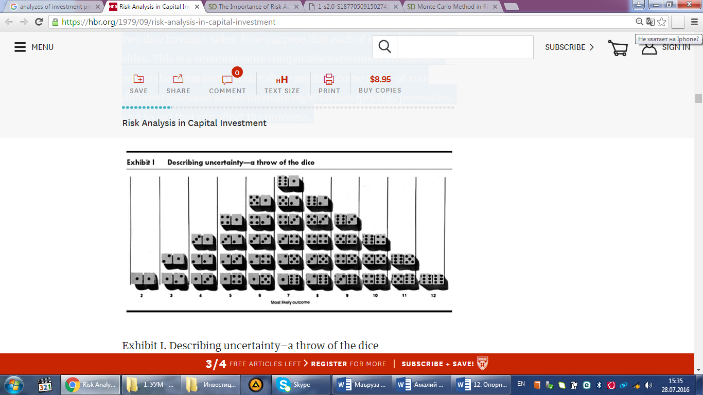
The expected rate of return represents only a few points on a continuous cure of possible combinations of future happenings. It is a bit like trying to predict the outcome in a dice game by saying that the most likely outcome is a 7. The description is incomplete because it does not tell us about all the other things that could happen. In Exhibit I, for instance, we see the odds on throws of only two dice having 6 sides. Now suppose that each of eight dice has 100 sides. This is a situation more comparable to business investment, where the company’s market share might become any 1 of 100 different sizes and where there are eight factors (pricing, promotion, and so on) that can affect the outcome.

Nor is this the only trouble. Our willingness to bet on a roll of the dice depends not only on the odds but also on the stakes. Since the probability of rolling a 7 is 1 in 6, we might be quite willing to risk a few dollars on that outcome at suitable odds. But would we be equally willing to wager $10,000 or $100,000 at those same odds, or even at better odds? In short, risk is influenced both by the odds on various events occurring and by the magnitude of the rewards or penalties that are involved when they do occur.

To illustrate again, suppose that a company is considering an investment of $1 million. The best estimate of the probable return is $200,000 a year. It could well be that this estimate is the average of three possible returns—a 1-in-3 chance of getting no return at all, a 1-in-3 chance of getting $200,000 per year, a 1-in-3 chance of getting $400,000 per year. Suppose that getting no return at all would put the company out of business. Then, by accepting this proposal, management is taking a 1-in-3 chance of going bankrupt.

If only the best-estimate analysis is used, however, management might go ahead, unaware that it is taking a big chance. If all of the available information were examined, management might prefer an alternative proposal with a smaller, but more certain (that is, less variable) expectation.

Such considerations have led almost all advocates of the use of modern capital-investment-index calculations to plead for a recognition of the elements of uncertainty. Perhaps Ross G. Walker summed up current thinking when he spoke of “the almost impenetrable mists of any forecast.”1

How can executives penetrate the mists of uncertainty surrounding the choices among alternatives?

Limited improvements

A number of efforts to cope with uncertainty have been successful up to a point, but all seem to fall short of the mark in one way or another.

1. More accurate forecasts

Reducing the error in estimates is a worthy objective. But no matter how many estimates of the future go into a capital investment decision, when all is said and done, the future is still the future. Therefore, however well we forecast, we are still left with the certain knowledge that we cannot eliminate all uncertainty.

2. Empirical adjustments

Adjusting the factors influencing the outcome of a decision is subject to serious difficulties. We would like to adjust them so as to cut down the likelihood that we will make a “bad” investment, but how can we do that without at the same time spoiling our chances to make a “good” one? And in any case, what is the basis for adjustment? We adjust, not for uncertainty, but for bias

For example, construction estimates are often exceeded. If a company’s history of construction costs is that 90% of its estimates have been exceeded by 15%, then in a capital estimate there is every justification for increasing the value of this factor by 15%. This is a matter of improving the accuracy of the estimate.

But suppose that new-product sales estimates have been exceeded by more than 75% in one-fourth of all historical cases and have not reached 50% of the estimate in one-sixth of all such cases? Penalties for such overestimating are very real, and so management is apt to reduce the sales estimate to “cover” the one case in six—thereby reducing the calculated rate of return. In so doing, it is possibly missing some of its best opportunities.

3. Revising cutoff rates

Selecting higher cutoff rates for protecting against uncertainty is attempting much the same thing. Management would like to have a possibility of return in proportion to the risk it takes. Where there is much uncertainty involved in the various estimates of sales, costs, prices, and so on, a high calculated return from the investment provides some incentive for taking the risk. This is, in fact, a perfectly sound position. The trouble is that the decision makers still need to know explicitly what risks they are taking—and what the odds are on achieving the expected return.

4. Three-level estimates

A start at spelling out risks is sometimes made by taking the high, medium, and low values of the estimated factors and calculating rates of return based on various combinations of the pessimistic, average, and optimistic estimates. These calculations give a picture of the range of possible results but do not tell the executive whether the pessimistic result is more likely than the optimistic one—or, in fact, whether the average result is much more likely to occur than either of the extremes. So, although this is a step in the right direction, it still does not give a clear enough picture for comparing alternatives.

5. Selected probabilities

Various methods have been used to include the probabilities of specific factors in the return calculation. L.C. Grant discussed a program for forecasting discounted cash flow rates of return where the service life is subject to obsolescence and deterioration. He calculated the odds that the investment will terminate at any time after it is made depending on the probability distribution of the service-life factor. After having calculated these factors for each year through maximum service life, he determined an overall expected rate of return.2

Edward G. Bennion suggested the use of game theory to take into account alternative market growth rates as they would determine rate of return for various options. He used the estimated probabilities that specific growth rates would occur to develop optimum strategies. Bennion pointed out:

“Forecasting can result in a negative contribution to capital budget decisions unless it goes further than merely providing a single most probable prediction…[with] an estimated probability coefficient for the forecast, plus knowledge of the payoffs for the company’s alternative investments and calculation of indifference probabilities…the margin of error may be substantially reduced, and the businessman can tell just how far off his forecast may be before it leads him to a wrong decision.”3

Note that both of these methods yield an expected return, each based on only one uncertain input factor—service life in the first case, market growth in the second. Both are helpful, and both tend to improve the clarity with which the executive can view investment alternatives. But neither sharpens up the range of “risk taken” or “return hoped for” sufficiently to help very much in the complex decisions of capital planning.

Sharpening the Picture

Since every one of the many factors that enter into the evaluation of a decision is subject to some uncertainty, the executives need a helpful portrayal of the effects that the uncertainty surrounding each of the significant factors has on the returns they are likely to achieve. Therefore, I use a method combining the variabilities inherent in all the relevant factors under consideration. The objective is to give a clear picture of the relative risk and the probable odds of coming out ahead or behind in light of uncertain foreknowledge.

A simulation of the way these factors may combine as the future unfolds is the key to extracting the maximum information from the available forecasts. In fact, the approach is very simple, using a computer to do the necessary arithmetic. To carry out the analysis, a company must follow three steps:

1. Estimate the range of values for each of the factors (for example, range of selling price and sales growth rate) and within that range the likelihood of occurrence of each value.

2. Select at random one value from the distribution of values for each factor. Then combine the values for all of the factors and compute the rate of return (or present value) from that combination. For instance, the lowest in the range of prices might be combined with the highest in the range of growth rate and other factors. (The fact that the elements are dependent should be taken into account, as we shall see later.)

3. Do this over and over again to define and evaluate the odds of the occurrence of each possible rate of return. Since there are literally millions of possible combinations of values, we need to test the likelihood that various returns on the investment will occur. This is like finding out by recording the results of a great many throws what percent of 7s or other combinations we may expect in tossing dice. The result will be a listing of the rates of return we might achieve, ranging from a loss (if the factors go against us) to whatever maximum gain is possible with the estimates that have been made.

For each of these rates we can determine the chances that it may occur. (Note that a specific return can usually be achieved through more than one combination of events. The more combinations for a given rate, the higher the chances of achieving it—as with 7s in tossing dice.) The average expectation is the average of the values of all outcomes weighted by the chances of each occurring.

We can also determine the variability of outcome values from the average. This is important since, all other factors being equal, management would presumably prefer lower variability for the same return if given the choice. This concept has already been applied to investment portfolios.

When the expected return and variability of each of a series of investments have been determined, the same techniques may be used to examine the effectiveness of various combinations of them in meeting management objectives.

Practical Test

To see how this new approach works in practice, let us take the experience of a management that has already analyzed a specific investment proposal by conventional techniques. Taking the same investment schedule and the same expected values actually used, we can find what results the new method would produce and compare them with the results obtained by conventional methods. As we shall see, the new picture of risks and returns is different from the old one. Yet the differences are attributable in no way to changes in the basic data—only to the increased sensitivity of the method to management’s uncertainties about the key factors.

Investment proposal

In this case, a medium-size industrial chemical producer is considering a $10 million extension to its processing plant. The estimated service life of the facility is ten years; the engineers expect to use 250,000 tons of processed material worth $510 per ton at an average processing cost of $435 per ton. Is this investment a good bet? In fact, what is the return that the company may expect? What are the risks? We need to make the best and fullest use of all the market research and financial analyses that have been developed, so as to give management a clear picture of this project in an uncertain world.

The key input factors management has decided to use are market size, selling prices, market growth rate, share of market (which results in physical sales volume), investment required, residual value of investment, operating costs, fixed costs, and useful life of facilities. These factors are typical of those in many company projects that must be analyzed and combined to obtain a measure of the attractiveness of a proposed capital facilities investment.

Obtaining estimates

How do we make the recommended type of analysis of this proposal? Our aim is to develop for each of the nine factors listed a frequency distribution or probability curve. The information we need includes the possible range of values for each factor, the average, and some idea as to the likelihood that the various possible values will be reached.

It has been my experience that for major capital proposals managements usually make a significant investment in time and funds to pinpoint information about each of the relevant factors. An objective analysis of the values to be assigned to each can, with little additional effort, yield a subjective probability distribution.

Specifically, it is necessary to probe and question each of the experts involved—to find out, for example, whether the estimated cost of production really can be said to be exactly a certain value or whether, as is more likely, it should be estimated to lie within a certain range of values. Management usually ignores that range in its analysis. The range is relatively easy to determine; if a guess has to be made—as it often does—it is easier to guess with some accuracy a range rather than one specific value. I have found from experience that a series of meetings with management personnel to discuss such distributions are most helpful in getting at realistic answers to the a priori questions. (The term realistic answers implies all the information management does not have as well as all that it does have.)

The ranges are directly related to the degree of confidence that the estimator has in the estimate. Thus certain estimates may be known to be quite accurate. They would be represented by probability distributions stating, for instance, that there is only 1 chance in 10 that the actual value will be different from the best estimate by more than 10%. Others may have as much as 100% ranges above and below the best estimate.

Thus we treat the factor of selling price for the finished product by asking executives who are responsible for the original estimates these questions:

• Given that $510 is the expected sales price, what is the probability that the price will exceed $550?

• Is there any chance that the price will exceed $650?

• How likely is it that the price will drop below $475?

Managements must ask similar questions for all of the other factors until they can construct a curve for each. Experience shows that this is not as difficult as it sounds. Often information on the degree of variation in factors is easy to obtain. For instance, historical information on variations in the price of a commodity is readily available. Similarly, managements can estimate the variability of sales from industry sales records. Even for factors that have no history, such as operating costs for a new product, those who make the average estimates must have some idea of the degree of confidence they have in their predictions, and therefore they are usually only too glad to express their feelings. Likewise, the less confidence they have in their estimates, the greater will be the range of possible values that the variable will assume.

This last point is likely to trouble businesspeople. Does it really make sense to seek estimates of variations? It cannot be emphasized too strongly that the less certainty there is in an average estimate, the more important it is to consider the possible variation in that estimate.

Further, an estimate of the variation possible in a factor, no matter how judgmental it may be, is always better than a simple average estimate, since it includes more information about what is known and what is not known. This very lack of knowledge may distinguish one investment possibility from another, so that for rational decision making it must be taken into account.

This lack of knowledge is in itself important information about the proposed investment. To throw any information away simply because it is highly uncertain is a serious error in analysis that the new approach is designed to correct.

Computer runs

The next step in the proposed approach is to determine the returns that will result from random combinations of the factors involved. This requires realistic restrictions, such as not allowing the total market to vary more than some reasonable amount from year to year. Of course, any suitable method of rating the return may be used at this point. In the actual case, management preferred discounted cash flow for the reasons cited earlier, so that method is followed here.

A computer can be used to carry out the trials for the simulation method in very little time and at very little expense. Thus for one trial 3,600 discounted cash flow calculations, each based on a selection of the nine input factors, were run in two minutes at a cost of $15 for computer time. The resulting rate-of-return probabilities were read out immediately and graphed. The process is shown schematically in Exhibit II

Data comparisons

The nine input factors described earlier fall into three categories:

1. Market analyses

Included are market size, market growth rate, the company’s share of the market, and selling prices. For a given combination of these factors sales revenue may be determined for a particular business.

2. Investment cost analyses

Being tied to the kinds of service-life and operating-cost characteristics expected, these are subject to various kinds of error and uncertainty; for instance, automation progress makes service life uncertain.

3. Operating and fixed costs

These also are subject to uncertainty but are perhaps the easiest to estimate.

These categories are not independent, and for realistic results my approach allows the various factors to be tied together. Thus if price determines the total market, we first select from a probability distribution the price for the specific computer run and then use for the total market a probability distribution that is logically related to the price selected.

We are now ready to compare the values obtained under the new approach with those obtained by the old. This comparison is shown in Exhibit III.

Exhibit III. Comparison of expected values under old and new approaches Note: Range figures in right-hand column represent approximately 1% to 99% probabilities. That is, there is only a 1-in-100 chance that the value actually achieved will be respectively greater or less than the range.

Valuable results

How do the results under the new and old approaches compare? In this case, management had been informed, on the basis of the one-best-estimate approach, that the expected return was 25.2% before taxes. When we run the new set of data through the computer program, however, we get an expected return of only 14.6% before taxes. This surprising difference results not only from the range of values under the new approach but also from the weighing of each value in the range by the chances of its occurrence.

Our new analysis thus may help management to avoid an unwise investment. In fact, the general result of carefully weighing the information and lack of information in the manner I have suggested is to indicate the true nature of seemingly satisfactory investment proposals. If this practice were followed, managements might avoid much overcapacity.

The computer program developed to carry out the simulation allows for easy insertion of new variables. But most programs do not allow for dependence relationships among the various input factors. Further, the program used here permits the choice of a value for price from one distribution, which value determines a particular probability distribution (from among several) that will be used to determine the values for sales volume. The following scenario shows how this important technique works.

Suppose we have a wheel, as in roulette, with the numbers from 0 to 15 representing one price for the product or material, the numbers 16 to 30 representing a second price, the numbers 31 to 45 a third price, and so on. For each of these segments we would have a different range of expected market volumes—for example, $150,000–$200,000 for the first,$100,000–$150,000 for the second, $75,000–$100,000 for the third. Now suppose we spin the wheel and the ball falls in 37. This means that we pick a sales volume in the $75,000–$100,000 range. If the ball goes in 11, we have a different price, and we turn to the $150,000–$200,000 range for a sales volume.

Most significant, perhaps, is the fact that the program allows management to ascertain the sensitivity of the results to each or all of the input factors. Simply by running the program with changes in the distribution of an input factor, it is possible to determine the effect of added or changed information (or lack of information). It may turn out that fairly large changes in some factors do not significantly affect the outcomes. In this case, as a matter of fact, management was particularly concerned about the difficulty in estimating market growth. Running the program with variations in this factor quickly demonstrated that for average annual growth rates from 3% to 5% there was no significant difference in the expected outcome.

In addition, let us see what the implications are of the detailed knowledge the simulation method gives us. Under the method using single expected values, management arrives only at a hoped-for expectation of 25.2% after taxes (which, as we have seen, is wrong unless there is no variability in the many input factors—a highly unlikely event).

With the proposed method, however, the uncertainties are clearly portrayed, as shown in Exhibit IV. Note the contrast with the profile obtained under the conventional approach. This concept has been used also for evaluation of product introductions, acquisition of businesses, and plant modernization

Comparing Opportunities

From a decision-making point of view one of the most significant advantages of the new method of determining rate of return is that it allows management to discriminate among measures of (1) expected return based on weighted probabilities of all possible returns, (2) variability of return, and (3) risks.

To visualize this advantage, let us take an example based on another actual case but simplified for purposes of explanation. The example involves two investments under consideration, A and B. With the investment analysis, we obtain the tabulated and plotted data in Exhibit V. We see that:

Investment B has a higher expected return than Investment A.

Investment B also has substantially more variability than Investment A. There is a good chance that Investment B will earn a return quite different from the expected return of 6.8%—possibly as high as 15% or as low as a loss of 5%. Investment A is not likely to vary greatly from the anticipated 5% return.

Investment B involves far more risk than does Investment A. There is virtually no chance of incurring a loss on Investment A. However, there is 1 chance in 10 of losing money on Investment B. If such a loss occurs, its expected size is approximately $200,000.

Clearly, the new method of evaluating investments provides management with far more information on which to base a decision. Investment decisions made only on the basis of maximum expected return are not unequivocally the best decisions.

Concluding Note

The question management faces in selecting capital investments is first and foremost: What information is needed to clarify the key differences among various alternatives? There is agreement as to the basic factors that should be considered—markets, prices, costs, and so on. And the way the future return on the investment should be calculated, if not agreed on, is at least limited to a few methods, any of which can be consistently used in a given company. If the input variables turn out as estimated, any of the methods customarily used to rate investments should provide satisfactory (if not necessarily maximum) returns.

In actual practice, however, the conventional methods do not work out satisfactorily. Why? The reason, as we have seen earlier in this article and as every executive and economist knows, is that the estimates used in making the advance calculations are just that—estimates. More accurate estimates would be helpful, but at best the residual uncertainty can easily make a mockery of corporate hopes. Nevertheless, there is a solution. To collect realistic estimates for the key factors means to find out a great deal about them. Hence the kind of uncertainty that is involved in each estimate can be evaluated ahead of time. Using this knowledge of uncertainty, executives can maximize the value of the information for decision making.

The value of computer programs in developing clear portrayals of the uncertainty and risk surrounding alternative investments has been proved. Such programs can produce valuable information about the sensitivity of the possible outcomes to the variability of input factors and to the likelihood of achieving various possible rates of return. This information can be extremely important as a backup to management judgment. To have calculations of the odds on all possible outcomes lends some assurance to the decision makers that the available information has been used with maximum efficiency.

This simulation approach has the inherent advantage of simplicity. It requires only an extension of the input estimates (to the best of our ability) in terms of probabilities. No projection should be pinpointed unless we are certain of it.

The discipline of thinking through the uncertainties of the problem will in itself help to ensure improvement in making investment choices. For to understand uncertainty and risk is to understand the key business problem—and the key business opportunity. Since the new approach can be applied on a continuing basis to each capital alternative as it comes up for consideration and progresses toward fruition, gradual progress may be expected in improving the estimation of the probabilities of variation.

Lastly, the courage to act boldly in the face of apparent uncertainty can be greatly bolstered by the clarity of portrayal of the risks and possible rewards. To achieve these lasting results requires only a slight effort beyond what most companies already exert in studying capital investments.

Retrospective Commentary

When this article was published 15 years ago, there were two recurrent themes in the responses of the management community to it: (1) how the uncertainties surrounding each key element of an investment decision were to be determined, and (2) what criteria were to be used to decide to proceed with an investment once the uncertainties were quantified and displayed.

I answered the latter question in an HBR sequel, “Investment Policies That Pay Off,” describing the relationships of risks and stakes to longer term investment criteria. This article, published in 1968, showed how risk analyses can provide bases for developing policies to choose among a variety of investment alternatives. Similar approaches were subsequently developed for investment fund portfolio management.

The analysis of uncertainty in describing complex decision-making situations is now an integral part of business and government. The elements of an investment decision—private or public—are subject to all the uncertainties of an unknown future. As the 1964 article showed, an estimated probability distribution paints the clearest picture of all possible outcomes. Such a description contains considerably more information than simplistic combinations of subjective best estimates of input factors. Best estimates are point estimates (there may be more than one—high, medium, low) of the value of an element of the investment analysis used for determining an outcome decision criterion, such as internal rate of return or present value of the investment.

Thus even where the conventional approach was used for the best estimate in a single-point determination for the statistically estimated expected values from a distribution of an element, the single-point approach was shown to be exceedingly misleading. In Exhibit III, a single-point best-estimate analysis gave an internal rate of return of 25.2%. And a risk analysis employing estimated frequency distributions of the elements showed that an average of possible outcomes, weighted by the relative frequency of their occurrences at 14.6%, was more realistic as well as significantly different. It presented a truer picture of the actual average expectation of the result of this investment (if it could be repeated over and over again).

The case was thus made, and the point of this result—that risk and uncertainty were more accurately defined by a simulation of input variables—was little questioned thereafter. Managements began to adopt some form of this procedure to examine some, if not all, significant investments where doubt existed about the risk levels involved. My sequel article attempted to demonstrate that if enough investments were chosen consistently on the basis of criteria related to these kinds of risk portrayals, the overall outcomes would stabilize around the desired expected value or best estimate of the criterion.

All this now seems simple and straightforward. Earlier it was falsely thought that risk analysis was aimed at eliminatinguncertainty, which was not worth doing at all since the future is so desperately uncertain. Thus in 1970 the Financial Times(of London) published an article intended to show the futility of risk analysis. It concerned a baker of geriatric biscuits who made an investment only to go bankrupt when his nursing home market precipitately disappeared with the death of its founder. The author cited as a moral, “Don’t put all your dough in one biscuit.”

It took a while for the points to diffuse through executive circles that (1) exactly such an analysis would have been just as bad, or worse, done via single-point subjective estimates, and (2) no one analytical technique could control future events, even with sensitive inputs and requirements for follow-up control to improve the odds as projected by the original risk analyses. But in the end, judgment would be required in both input estimation and decision.

I did not intend the article to be an argument in methodology but rather a cautionary note to examine the data surrounding an investment proposal in light of all the pervasive uncertainties in the world, of which business is simply one part. The years since 1964 have made it clear to me that this message should have been amplified and more emphatically insisted on in the article.

Had this point been clearer, the issue whether to take the risk and proceed with an investment might have been less troublesome. Had I been able to look with more prescience, I might have seen that the area of risk analysis would become routine in business and virtually universally adopted in public cost-benefit issues.

Cost-benefit analysis for public decisions is, of course, only a special form of investment analysis. Government issues that require decisions involving significant uncertainty are too numerous to catalog fully—energy, from both fossil and nuclear sources; chemical, drug, and food carcinogen hazards; DNA manipulation and its progeny of gene splicing.

The Three Mile Island nuclear accident brought home the fallibility of stating a risk analysis conclusion in simplistic terms. The well-known Rasmussen report on nuclear reactor safety, commissioned by the Nuclear Regulatory Commission, undertook what amounted to a risk analysis that was intended to provide a basis for investment decisions relating to future nuclear energy production. The Nuclear Regulatory Commission, in January 1979, disclaimed the risk estimates of that report; new studies to estimate risk are now underway. But there is also a school of thought saying we face too many risks each day to worry about one more.

A commonly stated estimate of the risk of a major nuclear power plant accident is 1 chance in 1,000,000 years. In the 1964 article, I portrayed the image of risk with a chart of the throws of two dice that would be required to give various outcomes—from two 1s to two 6s, each of these having a 1-in-36 chance of occurring. There should be no problem in visualizing or testing the meaning and the chances of any of the events pictured by these dice. And, although 1 in 1,000,000 is somehow presented as “mind boggling” compared with 1 in 36, and so unlikely to occur as to be beyond our ken, I suggest that it is just as simply visualized.

We simply need to use eight dice at once. If we chart all the possible outcomes for eight dice, as we did for the two, we find that the sum of 8 (or 48) can occur just one way—via all 1s (or all 6s). The odds of this occurring are roughly 1 in 1,680,000. Thus the visualization of such odds, and more important, the lesson we must learn about risk—which incidents like Three Mile lsland should teach us—is that what can happen will happen if we just keep at it long enough. Any of us can simulate a statistical picture of the estimated risks or even the complexities of the Rasmussen analysis with enough patience and enough dice (or a computer).

Incidentally, to make the eight dice act more like the odds of 1 in 1,000,000, simply mark any two “non-1” sides with a felt pen and count them as 1s if they turn up; the odds of getting all 1s become a little less than 1 in 1,100,000. And the chances of human error can be included by similarly marking other dice in the set. The difficulty is not in constructing such a simulation to portray the odds but in determining events that may lead to these odds and estimating the frequencies of their occurrence.

Risk analysis has become one with public policy. Without it, any important choice that leads to uncertain outcomes is uninformed; with it, properly applied and understood, the decision maker—business executive, government administrator, scientist, legislator—is better able to decide why one course of action might be more desirable than another.

1. “The Judgment Factor in Investment Decisions,” HBR March–April 1961, p. 99.

2. “Monitoring Capital Investments,” Financial Executive, April 1963, p. 19.

3. “Capital Budgeting and Game Theory,” HBR November–December 1956, p. 123