

Учебники / Hearing - From Sensory Processing to Perception Kollmeier 2007
.pdf38 |
M. Sayles et al. |
2.3Analyses
Spikes were analysed using a 50-ms windowed segment of the response with the analysis window slid in 12.5-ms steps. From these windowed spike train segments we calculated an all-order interspike interval distribution between pairs of non-identical sweeps. Such shuffled all-order interval histograms (referred to as shuffled autocorrelograms (SAC)) have been used previously to show temporal responses to broadband noise in auditory nerve fibres (Louage et al. 2004).
3Results
The preliminary results reported in this paper come from the responses of 67 units in the VCN (8 Primary-Like, 15 Transient Chopper, 29 Sustained Chopper, 6 Onset (On-I and On-L) and 9 Low-BF phase-locking units). In most cases a range of frequency sweeps were played. Examples from three units are shown below. The plots show windowed normalised SAC functions.
In Fig. 2 we show the responses of a low-BF unit to a harmonic complex sweep with an F0 transition from 100 to 200 Hz over 500 ms. There is a clear peak in panel A at delays corresponding to the F0 throughout the response. There are also obvious peaks at shorter delays corresponding to delays appropriate for the second and third harmonics. The unit BF is 352 Hz; thus initially the third harmonic of the 100 to 200-Hz sweep would be dominant within the unit’s filter, with the second harmonic rapidly taking over as the dominant component. Approximately mid-way through the response the unit seems to respond predominantly to the fundamental component. With increasing levels of reverberation (Fig. 2B–D) the temporal representation of the stimulus remains clearly visible as peaks in the SAC, although the response to the third and second harmonics appears to be spread to later time points. We have observed similar responses from nine units with BFs in the range 200–500 Hz.
The responses of a Transient Chopper unit (BF = 2.34 kHz) are shown in Fig. 3. Again there is a clear representation of the stimulus in the dry condition, with peaks in the SAC corresponding to the stimulus fundamental. The peaks become much sharper as the stimulus periodicity enters this unit’s range of preferred periodicities. The BF of this unit is 2.34 kHz; hence it is responding to envelope periodicity resulting from beating between several unresolved harmonics within the peripheral filter. There is still a representation of the F0 transition in the 32-cm condition, although at 125 cm and 500 cm this representation has disappeared with the SACs tending towards unity, indicating the presence of uncorrelated spike times. This response pattern is typical of our population of units of all response types (except Onset- I) with BFs above approximately 1 kHz.

The Effect of Reverberation on the Temporal Representation of the F0 |
39 |
Low frequency Phase-locking unit (1270011)
BF = 352 Hz
Left: SACs
Binwidth = 50 s
Below: PSTH Binwidth = 0.2 ms
250 presentations of a 50-ms tone at BF, 50 dB above unit threshold
Fig. 2 Windowed normalised SACs of the response to a harmonic complex sweep with F0 100–200 Hz from a Low-BF unit: A the response to the dry stimulus and panels; B–D responses to the same stimulus after convolution with impulse responses at source-to-receiver distances as indicated in each panel. The scale along the ordinate in each case indicates the time through the stimulus.
The responses from a unit classified as Onset-I are shown in Fig. 4. This unit exhibits an almost perfect representation of the F0 transition in the dry condition. However, the addition of even very mild reverberation (32 cm) results in the almost complete abolition of a driven response. By 500 cm the raster plots in Fig. 4B show only spikes at stimulus onset. We have observed two units classified as On-I with this response pattern. Onset-L units give responses similar to those shown for the transient chopper neuron in Fig. 3.
4Discussion
We have shown that units responding to low-numbered resolved harmonics (Fig. 2) maintain a representation of the F0 in their interspike intervals even with relatively severe reverberation. In contrast the same representation in units responding to envelope modulation appears to be degraded with even relatively mild reverberation.

40 |
M. Sayles et al. |
Transient Chopper unit (1275006)
BF = 2.34 kHz
Chopping freq.=500 Hz
Below: PSTH Binwidth = 0.2 ms
250 presentations of a 50-ms tone at BF, 50 dB above unit threshold
Fig. 3 Same format as Fig. 2 but for a Transient Chopper unit in response to the 100 to 200-Hz sweep
Fig. 4 A Windowed SAC function from the responses of an On-I unit (BF = 3.41 kHz) to a harmonic complex sweep stimulus with an F0 of 250–500 Hz. B Dot raster plots for the responses to the dry condition (top) and the three reverberation conditions
The Effect of Reverberation on the Temporal Representation of the F0 |
41 |
The breakdown of the temporal response in high frequency channels is likely due to the randomisation of the phase relationships between unresolved partials of the complex. This is further supported by the fact that low frequency channels showing responses to resolved components appear more resistant to the effects of reverberation with the main effect in these units being due to the smearing of the acoustic spectrum through time. Our On-I units’ responses to the reverberant conditions are similar to those in response to random phase harmonic complexes (Evans and Zhao 1998).
A major attraction of temporal theories of pitch processing (based largely on the autocorrelation approach) is that the same neuronal operation (i.e. counting of coincidences) applies equally well for both resolved and unresolved partials of a complex. Others have argued for a two-mechanism hypothesis, invoking some pattern recognition scheme for resolved regions and temporal processing for unresolved regions (e.g. Shackleton and Carlyon 1994). Despite the wealth of psychophysical evidence concerning the perception of vowels and other speech sounds under reverberant conditions, no study to our knowledge has specifically addressed the issue of the effect of reverberation on pitch perception when listening to either resolved or unresolved harmonics.
Our results suggest that in the presence of reverberation the use of temporal information may be limited to frequency channels containing resolved harmonics. These results are interesting in light of psychophysical evidence that in the presence of reverberation and a modulated F0 contour listener’s ability to perceptually segregate two competing sound sources with different F0s is compromised. In order to segregate sounds on the basis of an F0 difference it is necessary for a central processor to estimate the pitch of at least one of the competing sources, in order to either enhance the target sound, or to cancel the interfering sound (de Cheveigné et al. 1995). Based on our results it seems likely that if the listener is making use of higher, unresolved, harmonics to estimate the pitch of the interfering sound in the presence of reverberation, the cancellation of this sound would be difficult.
Ackowledgements. This work was supported by the BBSRC and the Wellcome Trust. We thank the Frank Edward Elmore and James Baird funds of the Cambridge MB/PhD programme for supporting one of the authors, MS.
References
Bleeck S, Sayles M, Ingham NI, Winter IM (2006) The time course of recovery from suppression and facilitation from single units in the mammalian cochlear nucleus. Hear Res 212:176–184 Culling JF, Summerfield Q, Marshall DH (1994) Effects of simulated reverberation on the use of binaural cues and fundamental-frequency differences for separating concurrent vowels.
Speech Commun 14:71–95
de Cheveigné A, McAdams S, Laroche J, Rosenberg M (1995) Identification of concurrent harmonic and inharmonic vowels: a test of the theory of harmonic cancellation and enhancement. J Acoust Soc Am 97:3736–3748
42 |
M. Sayles et al. |
Evans EF, Zhao W (1998) Periodicity coding of the fundamental frequency of harmonic complexes: physiological and pharmacological study of onset units in the ventral cochlear nucleus. In: Psychophysical and physiological advances in hearing. Proceedings of the 11th international symposium on hearing, 1997. Whurr, London
Knudsen VO (1929) The hearing of speech in auditoriums. J Acoust Soc Am 1:56–82
Louage DH, van der Heijden M, Joris PX (2004) Temporal properties of responses to broadband noise in the auditory nerve. J Neurophysiol 91:2051–2065
Merrill EG, Ainsworth A (1972) Glass-coated platinum tipped tungsten microelectrodes. Med Biol Eng 10:662–672
Nàbeˇlek AK, Letowski TR, Tucker FM (1989) Reverberant overlapand self-masking in consonant identification. J Acoust Soc Am 86:1259–1265
Santon F (1976) Numerical prediction of echograms and of the intelligibility of speech in rooms. J Acoust Soc Am 59:1399–1405
Shackleton TM, Carlyon RP (1994) The role of resolved and unresolved harmonics in pitch perception and frequency modulation discrimination. J Acoust Soc Am 95:3529–3540
Watkins AJ (2005) Perceptual compensation for effects of reverberation in speech identification. J Acoust Soc Am 118:249–262
Comment by Langner
Your results may be explained by the way pitch information is mapped in the inferior colliculus (IC). As we have shown by single unit recordings as well as by functional mapping with the 2-Deoxyglucose method, a harmonic sound is represented by a column of activated neurons parallel to the tonotopic gradient. The activation of low frequency neurons is due to resolved harmonics, possible distortion products, and across frequency activation in the IC. The activation of neurons with higher CFs requires periodicity coding (according to my model by a cross-correlation of envelope periodicity with resolved harmonics). If you cut the lowest harmonics from the stimulus, the neuronal column is still (partly) activated, because periodicity coding works for higher harmonics. If you destroy periodicity information by reverberation, the column is (partly) activated by resolved harmonics alone. In either case, pitch remains encoded in the same way, by the same neuronal column in the IC.

6 Spectral Edges as Optimal Stimuli for the Dorsal Cochlear Nucleus
SHARBA BANDYOPADHYAY1, ERIC D. YOUNG1, AND LINA A. J. REISS2
1Introduction
The principal neurons of the dorsal cochlear nucleus (DCN) form one of several parallel pathways through the brainstem from the cochlear nucleus to the inferior colliculus (Rouiller 1997). Unlike the neurons of the ventral cochlear nucleus, DCN principal cells give strongly non-linear responses to sound (Nelken et al. 1997; Yu and Young 2000), meaning that models of DCN neurons often do not predict the responses to complex sounds. Such nonlinearity is typical of auditory neurons (e.g. Eggermontet al. 1983; Machenset al. 2004) and poses difficulties for studies of the representation of sound in the brain, because it is not possible to obtain a comprehensive view of the representation of sound by such nonlinear neurons.
In the case of the DCN, information about function has been provided by behavioral experiments in which the nucleus or its output tract were lesioned (e.g. May 2000), leading to deficits in sound localization. In addition, the DCN receives inputs from various non-auditory sources, including the somatosensory system (Davis et al. 1996; Shore 2005) and these seem to have specifically to do with the position of the external ear in cats (Kanold and Young 2001). These results are consistent with the finding that DCN neurons in the cat respond sensitively with inhibition to the acoustic notches in the head-related transfer functions of the cat external ear (reviewed in Young and Davis 2001). Together, these data suggest a role in sound localization for the DCN, especially in localization based on spectral cues.
2Spectral Notches and Spectral Edges
However, stimuli like acoustic notches and head-related transfer functions are complex, with multiple components (Fig. 1A); it is unclear exactly which components are important to DCN responses. Two approaches to this question are
1Biomedical Engineering and Center for Hearing and Balance, Johns Hopkins University, Baltimore, USA, eyoung@bme.jhu.edu, sbandyop@bme.jhu.edu
2Speech Pathology and Audiology, University of Iowa, Iowa City, USA, lina-reiss@uiowa.edu
Hearing – From Sensory Processing to Perception
B. Kollmeier, G. Klump, V. Hohmann, U. Langemann, M. Mauermann, S. Uppenkamp, and J. Verhey (Eds.) © Springer-Verlag Berlin Heidelberg 2007
44
A
Gain re free-field, dB
S. Bandyopadhyay et al.
20 |
|
|
|
|
10 |
|
|
|
|
0 |
|
|
|
|
−10 |
158 |
Az., |
|
|
|
|
|
||
−20 |
−158 |
El. |
|
|
2 |
|
5 |
20 |
40 |
|
|
|
Frequency, kHz |
|
B |
C |
|
|
|
|
|
|
70 |
|
|
|
|
SPL |
60 |
|
|
|
|
50 |
|
|
|
|
|
dB |
40 |
|
|
|
|
level, |
|
|
|
|
WBI |
30 |
|
|
|
|
Sound |
|
|
|
||
II |
20 |
|
|
|
|
|
|
|
|
|
|
|
|
10 |
|
|
|
ANF |
|
0 |
|
|
|
|
1 |
3 |
10 |
30 |
|
|
|
||||
|
|
|
Frequency, kHz |
|
|
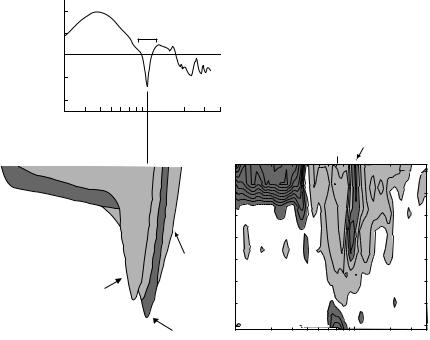
Fig. 1 A Cat head-related transfer function. The bracket at 10 kHz shows 0.5 oct. B Model of the tone response maps of DCN type IV neurons. C Response map of a DCN type IV neuron. Dark gray is excitatory, light gray is inhibitory. Contours are iso-rate, spaced at 12 spikes/s. Responses within 5 spikes/s of spontaneous rate are suppressed. Line at top marks the BF
taken in this chapter: first, responses to notches with systematic variation of the notch width and center frequency suggest that the upper-frequency edge of the notch is the important aspect (Middlebrooks 1992; Reiss and Young 2005). Second, a new approach to finding the optimal stimulus for a neuron is used to show that a rising spectral edge located at the neuron’s best frequency (BF) is often the optimal stimulus for a DCN principal cell.
The responses of a DCN principal cell (type IV neuron) to tones are summarized in the response map in Fig. 1C. As for all the data in this paper, these data are from a well-isolated single neuron in an unanesthetized, decerebrate cat. Such neurons are excited by frequencies near the best frequency (BF) at low sound levels (near 7 kHz at 0 dB SPL) and usually also at frequencies above BF (≈10 kHz) at higher sound levels (arrow). Other excitatory areas may be present, but the inhibitory area centered on BF and the second inhibitory area above BF (>10 kHz) are characteristic. The model in Fig. 1B provides an explanation for DCN response maps (Blum and Reed 1998). It consists of excitatory
Spectral Edges as Optimal Stimuli for the Dorsal Cochlear Nucleus |
45 |
input from auditory nerve fibers (ANF, dark gray) with strong inhibitory inputs from so-called type II neurons (light gray) and weaker inhibition from a second source (WBI; Nelken and Young 1994). The BF of the type II inhibitory input is shifted to a frequency below the neuron’s (and the ANF’s) BF and the inhibitory input has a higher threshold (Voigt and Young 1990), resulting in the major excitatory and inhibitory features in the response map.
Figure 1A shows a typical cat head-related transfer function with a spectral notch positioned at the BF of the model (dashed line). This is the spectrum at the eardrum for a broadband noise presented in free field from 15˚ azimuth, −15º elevation. Because of the offset in their BFs, this notch would activate the excitatory input without activating the inhibitory input, leading to a strong response from the model. These features of the response map suggest that the upper edge of a notch might be a strong stimulus for DCN type IV neurons.
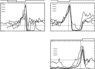
Responses to spectral notches of a type IV neuron are shown in Fig. 2 in the form of discharge rate (ordinate) as the notch is moved in frequency (abscissa; Reiss and Young 2005). The abscissa is the frequency of the rising edge of the stimulus in each case. Figure 2A shows that notches of various
A |
|
1 |
0.5 |
|
B |
|
100 |
0.125 oct. |
13 dB |
100 |
|
|
|
0.25 oct. |
spect. level |
|
|
sp./s. |
80 |
0.5 oct. |
|
|
80 |
1 oct. |
|
|
|||
|
|
|
|
||
60 |
|
|
|
60 |
|
Rate, |
|
|
|
||
40 |
|
|
|
40 |
|
|
|
|
|
|
|
|
20 |
|
|
|
20 |
|
0 |
|
|
|
0 |
10 |
20 |
30 |
40 |
|
Upper edge freq., kHz |
|
|
3 dB |
|
0.5 octave |
13 dB |
|
notchwidth |
23 dB |
|
|
|
|
|
33 dB |
|
|
20 |
30 |
40 |
Upper edge freq., kHz
|
C |
|
|
|
|
100 |
0.5 octave |
|
|
|
bandwidth |
|
||
|
|
|
||
sp./s. |
80 |
|
3 dB |
|
|
|
13 dB |
|
|
60 |
|
23 dB |
|
|
Rate, |
|
|
33 dB |
|
40 |
|
|
|
|
|
|
|
|
|
|
20 |
|
|
|
|
0 |
10 |
20 |
30 |
|
|
|||
Lower edge freq., kHz
Fig. 2 Rate responses of a DCN neuron to notches (A,B) or noise bands (C) moved in frequency. Abscissae show the frequency of the rising edge of the notch or band. Passbands were 30 dB above stopbands. Sound levels are passband spectrum level, dB re 20 Pa/Hz1/2. The spectra giving maximum rate are shown above the plots. Horizontal dashed line is average spontaneous rate, vertical dashed line is BF
46 |
S. Bandyopadhyay et al. |
widths (see the legend) produce a strong excitatory response when the upper-frequency edge of the notch is near BF (vertical dashed line) and inhibition when the notch is centered on BF (when the upper edge frequency is just above BF). This pattern of response remains across a range of sound levels (Fig. 2B, for 1/2 octave notches). It is also observed when the stimulus is a noise band, but in this case is associated with the lower-frequency edge of the band, on the abscissa in Fig. 2C.
3Finding the Optimal Stimulus
A useful approach to understanding the sensory representation by nonlinear neurons is to search for optimal stimuli (e.g. deCharms et al. 1998; O’Connor et al. 2005). The characteristics of a neuron’s optimal stimulus provide a functional definition of the signal processing being done by the neuron. The optimum can be the stimulus giving the highest discharge rate or it can be the stimulus about which the neuron provides the most information in some sense. In this chapter the optimum is the maximum discharge rate.
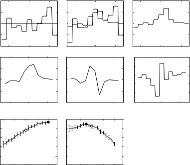
The problem of finding the optimum is not well defined and must usually be limited to some class of stimuli. Here, the stimulus class is random spectral shape stimuli (RSS; Yu and Young 2000; Young and Calhoun 2005) and the optimum spectral shape is sought. RSS stimuli consist of sums of random-phase tones spaced at 1/64 octave intervals over a several-octave frequency range; the tones are gathered into sets of 8 in 1/8 octave bins. The total power in each bin, in dB relative to a reference stimulus, varies pseudo-randomly with an approximately Gaussian distribution and a standard deviation of 1.5–12 dB. These stimuli have minimal envelope fluctuations and the effects of the temporal envelope are not considered. Figure 3A shows examples of the spectra of RSS stimuli.
The optimization proceeds by changing the spectral shape iteratively, guided by the Fisher information matrix F of the responses (Cover and Thomas 1991). The i–jth term in the Fisher matrix is
Fij =E > |
2 |
ln p (r ; q) |
2 |
ln p (r ; q)H. |
(1) |
2qi |
2q j |
where p(r; q) is the pdf of discharge rate r given the stimulus parameters q, the amplitudes (dB) of the stimulus in the 11 RSS bins centered on BF. Fij is the sensitivity of the neuron’s rate response to simultaneous changes in the stimulus amplitude in the ith and jth bins, in the sense that the inverse of the Fisher matrix is the covariance matrix of the minimum-variance unbiased estimator of q based on r (the Cramér-Rao bound). The Fisher matrix can be computed from rate data using the following approximation (Johnson et al. 2001):
|
1 |
T |
(2) |
D ( p (r; q + dq) || p (r; q)) . |
|
dq F dq |
|
2 ln 2 |
Spectral Edges as Optimal Stimuli for the Dorsal Cochlear Nucleus |
47 |
A
atten.dB |
40 |
|
|
Level, |
50 |
|
C |
|
−0.5 |
0 |
0.5 |
|
1 |
|
|
|
||
eigenvector |
|
|
|
||
0.5 |
|
|
|
||
0 |
|
|
|
||
|
|
|
|
||
Largest |
−0.5 |
|
|
|
|
−1 |
−0.5 |
0 |
0.5 |
||
|
|
|
|
B |
|
|
|
|
|
|
|
* |
|
|
|
* |
* |
|
|
|
|
* |
|
|
−0.5 |
0 |
0.5 |
−0.5 |
0 |
0.5 |
|
|
|
D |
|
|
|
|
|
30 |
* |
|
|
|
|
|
|
|
|
|
|
40 |
|
|
|
|
|
50 |
* |
|
|
|
|
|
|
|
−0.5 |
0 |
0.5 |
−0.5 |
0 |
0.5 |
E |
|
|
|
|
|
|
(sp/s) |
200 |
|
|
|
|
|
|
|
|
|
|
|
|
Rate |
100 |
|
|
|
|
|
|
|
|
|
|
|
|
|
0 |
−8 |
−4 |
0 |
4 |
8 |
Octaves re BF
−8 |
−4 |
0 |
4 |
8 |
Eigenvector multiplier, dB
Fig. 3A–E Finding the optimal stimulus shape. The abscissae in A–D are frequency, in octaves re BF. The ordinate scale in D is level in dB attenuation as in A,B
where D( ) is the so-called KL distance between the pdfs of the rate response to stimulus vectors q + δ q and q and the approximation is good for small δ q. The change δq in the stimulus that gives the largest change in the KL distance in Eq. (2) is parallel to the eigenvector with the largest eigenvalue emax, i.e.
δqmax = Aemax, where A is a constant. It can be shown from a model of RSS responses that, for small δ q, this also gives the largest change in discharge
rate. Thus the rate optimization proceeds by estimating F in the vicinity of a reference stimulus q, then finding the δ q that produces the largest rate change by empirically finding the value of A (limited to ±8 dB) such that δqmax = A emax gives the largest rate change. The reference stimulus is then changed to q + δqmax and the process is repeated. The process terminates when the reference q is a rate maximum, as judged from a local quadratic model of the dependence of rate on δ q. This process is done on-line and typically requires ~1 h and three iterations.
The Fisher matrix is estimated from rate responses r to a large number of different perturbations δq around the reference stimulus, giving many simultaneous linear algebraic equations like Eq. (2) with the terms of F as the unknowns. The KL distance is computed from the mean rates, assuming that r is Poisson.