Учебники / Hearing - From Sensory Processing to Perception Kollmeier 2007

was presented (Pastore and Sorkin 1971). Still others showed that it is possible to simultaneously tune several listening bands on different frequencies or even on a frequency the listener was never physically presented with, only instructed to imagine (Schlauch and Hafter 1991). Thus, it seems that listening bands exist in the memory of listeners and linger on for long periods of time in quiet or in the absence of hearing another signal with a different, salient pitch (Demany and Semal 2005).

Recent physiological data also suggest that tones give rise to activity patterns the excitatory and inhibitory contours of which outlast the presence of the tone itself (Fritz et al. 2005). It could well be that the existence of listening bands may stem from these contours and may underlie behavioral findings on listeners’ ability to shift the frequency focus. However, if the new frequency focus is in one of the inhibitory bands flanking the excitatory band of the previous frequency focus, the build-up of new excitation takes time and thus the shift of the listening band should not be instantaneous. Unfortunately, important questions related to the timing of this phenomenon have not been asked: how long does it take to establish listening bands, how long do they last in absence of a stimulus, and how long does it take to establish a new listening band when the frequency of a tonal stimulus changes? The present study attempts to answer these questions which, it seems, have important physiological implications. The hypothesis to be tested in a psychophysical experiment is that when a tone of different frequency follows one of a given frequency, it will be perceived with a delay because it first has to overcome the inhibitory effect of the previous tone – a process which takes time.

2Methods

Since the delay stated by the hypothesis is not expected to be longer than a few milliseconds, the question to ask is whether there is a psychophysical method sensitive enough to measure time intervals so short. Earlier work (Divenyi and Danner 1977) showed that, in the 20to 50-ms range, 4–6% differences of unfilled time intervals marked by brief tone or noise bursts can be reliably discriminated. In the present study, we used this ability to have listeners compare a 40-ms onset-to-onset time interval marked by two tone bursts of frequency f1 to a time interval marked by one tone burst of frequency f1 and another of frequency f2. The comparison was done using the Method of Adjustment: the listener was instructed to adjust the second time interval between the f1 and f2 frequency markers to match the first interval, the 40-ms standard between the two f1 frequency markers, as shown in the top diagram of Fig. 1. The difference between frequencies f1 and f2 was varied from condition to condition such that the geometric mean remained constant at 1 kHz. The tone bursts of 20-ms nominal duration (and 15-ms half-power duration) were shaped with a 2-ms onset and a 10-ms offset; their envelope

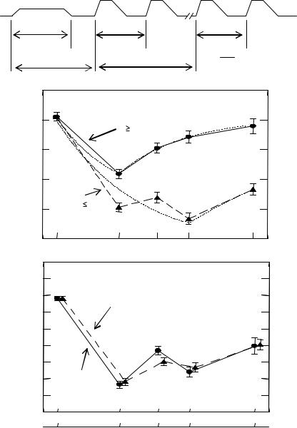
Fig. 1 The stimulus from Experiment 1 (top) and the perceptual error in judging the second time interval (bottom)

was rounded to minimize transients. The time separating the onset of the first burst of the two observation intervals was 600 ms; the trials proceeded at a 2.5-s rate, thus allowing the subject a response time of close to 2 s. That is, the diagram should be imagined to be repeating with cycle of 2.5 s. Stimuli were presented monaurally to the subject’s right earphone (TDH-49 in MX/AR cushions) at 86 dB SPL. A run was terminated when the subject indicated that the two intervals were perceived identical. The reported data represent the average of 48–96 adjustments for each subject in each experimental condition. Subjects were normal-hearing young volunteers.

3Results

3.1Experiment 1

The averaged duration of the second time interval judged by our subjects to be identical to the first are illustrated in Fig. 1 as “perceptual error”: the difference between the adjusted second observation interval and the 40-ms

standard as a function of frequency difference ∆f in Hertz and in octaves. In this experiment, the frequency f2 was always equal to or lower than f1, i.e., the frequency change within each trial went in a downward direction. One notices that the error is positive when ∆f is zero, an outcome we attribute to the “time order error” (Helson and Himelstein 1955) frequently observed when comparing two identical stimuli. We assume for the present data that this error does not change across frequency differences, that is, the temporal judgment error due to frequency difference can be attributed to another source. This source appears to have to do with frequency f2 influencing the listeners’ time judgments such that they adjusted the interval shorter than 40 ms. This perceptual error takes a “W” shape with two minima (i.e., maximum error points): one when ∆f is about 1/3 octave and the other when it is around 2/3 octave. In addition, although at frequency differences of 1 octave and larger the time judgment error essentially vanishes, its uncertainty (measured as the standard error of the mean shown in the error bars) increases several fold.

On the whole, the results confirm our hypothesis: the negative perceptual errors suggest that the perceived onset of the burst with the f2 frequency occurred a few ms later than its physical onset, possibly because it had to overcome the inhibitory contour of the preceding burst of frequency f1. Interestingly, the subjects seemed to be very certain when adjusting this second time interval shorter than the first, as indicated by the small degree of uncertainty. The inhibitory contours of f1 do not appear to extend beyond 2/3 octave, as if the listening band was “shifted” up to that frequency difference but for differences larger than this limit a “switching” (Swets’ [1963] term) between listening bands took place.

However, what could account for the dual error maxima? Indeed, this non-monotonicity is difficult to explain unless one assumes that the inhibitory contours of the listening band are long-lasting, that is, persisting at least for the duration of the 2-s interval that separates the last (f2) burst of a trial and the first burst (f1) of the next – in which case the onset of this first burst of frequency f1 will be perceived after a delay necessary to overcome the inhibition around the burst of frequency f2, i.e., the last tone of the preceding trial. However, unlike the downward frequency change in the second observation interval from f1 to f2, that frequency change moves in an upward direction. If the inhibitory contours around a certain frequency do not spread to the same extent above and below, as in masking (Shannon 1976) and in the ventral cochlear nucleus (Rhode and Greenberg 1994), then we would expect to obtain the “W”- shaped result.

Granted, this explanation is based on two corollary hypotheses – (1) that the inhibition lingers on far beyond the cessation of a tone and (2) that it spreads farther in one direction on the frequency axis than in the other. If these hypotheses are true, they also bring with them the consequence that the perceptual errors observed in Experiment 1 actually represent the

sum of two delays: one that makes the second observation interval longer by delaying its second burst (of frequency f2), and one that makes the first observation interval shorter by delaying its first burst (of frequency f1). Fortunately, both hypotheses are testable with a modification of the stimulus used in Experiment 1.

3.2Experiment 2

As it turns out, the above hypotheses are easily tested by introducing two modifications to the stimulus: (1) have a tone of frequency f1 precede the first burst of the trial, so that, if the inhibitory contours of the f2 tone in the previous trial must be overcome when the frequency of the tone burst changes back to f1, such a “disinhibition” occurs before the 40-ms interval is presented, and (2) add conditions in which the second observation interval’s frequency change goes upward. These modifications should also measure the perceptual error due to the f2 burst overcoming the inhibitory contours of the f1 burst in the second observation interval alone, rather than the two summed effects we predicted that the results of Experiment 1 reflect. The top diagram of Fig. 2 shows the stimulus: it differs from that of Experiment 1 in that it has a long (150-ms) tone of frequency f1 precede the stimulus proper. This added “cueing” tone has gradual (50-ms) onset and offset and is presented at a level 15 dB below the stimulus, in order for it not to interfere with the fine temporal discrimination needed to compare the 40-ms standard and the variable time intervals.

Averaged results of the subjects are shown in the body of Fig. 2. The top data graphs illustrate those separately for the downward and upward f1-to- f2 frequency change and indicates two effects: (1) the perceptual errors of time adjustments are about half the size of those observed in Experiment 1, and (2) the largest error for the upward frequency change occurs at a frequency difference of about 2/3 octave, i.e., about twice the ∆f at which the largest error for the downward frequency change is observed (~1/3 octave). In other words, the data confirm the two corollary hypotheses. To test more rigorously the hypothesis that the Experiment 1 results were induced by two frequency changes within any single trial (one downward and one upward), we computed for each ∆f value the sum of the perceptual errors observed at the downward and the upward frequency changes in Experiment 2 and compared it with the results of Experiment 1 averaged for the three subjects. The bottom graph of Fig. 2 in which this comparison is displayed indicates that the summed results of Experiment 2 and the results of Experiment 1 are essentially identical. The most surprising finding that derives from this equivalence is that, in Experiment 1, the putative inhibitory effects of the tone of frequency f2 appear to have been still in effect when the first tone of frequency f1 was presented in the next trial – i.e., over a period of about 2 s.

The two experiments have generated results consistent with our hypotheses and in general agreement with physiological observations. We are thus inclined to think that establishing listening bands is a dynamic process that may reflect excitatory and inhibitory profiles at diverse stages of the auditory system.

3.3A Model of Listening Band Dynamics

Excitatory build-up and decay in the auditory nerve expressed as discharge rate have been shown to obey an exponential law (Smith 1977). The model we explored follows this law and represents t∆ƒ, the time required to shift the listening band from a first frequency to a second located ∆ƒ Hz (or octaves) away as

where A is a weighting constant that affects the inhibitory and the disinhibitory processes to the same degree, a and b are the growth constants of the inhibitory and disinhibitory processes, respectively, ƒlim is the frequency difference at which the disinhibitory process begins, and u is the unit step function. The model constants were calculated using a nonlinear regression and the individual subjects’ data. The model output is shown as the dotted lines in the top graph of Fig. 2.

4Discussion

The results’ general agreement with the model suggests that the buildup of listening bands, taking up to 2–4 ms at the maximum frequency change at which this buildup is observed, may be related to the excitatory buildup when the stimulus frequency is one that falls in the inhibitory area generated by a previously presented different frequency. Such short delay for the buildup of excitation also suggests that the process responsible for it is likely to take place in, or close to, the auditory periphery. Our data also show that past this frequency limit the buildup diminishes and eventually vanishes, suggesting that the new excitatory process encounters less, and eventually no, inhibition: it builds up a contour around a frequency not affected by the previous tone’s response contours. However, the moment of the onset of this new tone is not integrated efficiently with that of the old – hence the increased variability at frequency differences approaching the octave – consistent with what has been observed for the discrimination of gaps between spectrally different markers (Divenyi and Danner 1977).

However, the results also raise many questions. What would be the buildup time of response contours generated by broad-band instead of puretone markers? If the buildup delay truly originates at the periphery, does this

mean that shifting listening bands across ears would not result in any observable delay? Also, since the inhibitory sidebands are intensity dependent, would changing the intensity of the markers influence the buildup delay? If data collected in other experiments were to answer these questions in a way still consistent with the original hypotheses, these new experiments would strengthen the view that listening bands develop dynamically. In absence of such data our knowledge about changing the frequency focus of listening bands has not been significantly advanced.

5Conclusion

Listening bands have an itch: Will the ear scan? Will it switch? Yet, unless one bets

on wisdom by Swets (1963), knows this no son of a ....

Acknowledgments. The authors thank Ira Hirsh, James Saunders, and Steven Greenberg for many helpful comments on earlier versions of the manuscript, and the assistance of JC Sander for data analysis. The research was supported by the National Institutes of Health and the Department of Veterans Affairs.

References

Demany L, Semal C (2005) The slow formation of a pitch percept beyond the ending time of a short tone burst. Percept Psychophys 67:1376–1383

Divenyi PL, Danner WF (1977) Discrimination of time intervals marked by brief acoustic pulses of various intensities and spectra. Percept Psychophys 21:125–142

Evans EF (2001) Latest comparison between physiological and behavioural frequency selectivity. In: Breebart DJ, Houtsma AJM, Kohlrausch A, Prijs VF, Schoonhoven R (eds), Physiological and psychological bases of auditory function. Shaker Publishing, Maastricht, the Netherlands, pp 382–387

Fritz J, Elhilali M, Shamma S (2005) Active listening: task-dependent plasticity of spectrotemporal receptive fields in primary auditory cortex. Hear Res 206:159–176

Greenberg GZ, Larkin WD (1968) Frequency-response characteristics of auditory observers detecting signals at a single frequency in noise: the probe-signal method. J Acoust Soc Am 44:1513–1523

Helson H, Himelstein P (1955) A short method for calculating the adaptation-level for absolute and comparative rating judgments. Am J Psychol 68:631–637

Moore BCJ (2003) Psychology of hearing, 5th edn. Academic Press, San Diego

Pastore RE, Sorkin RD (1971) Adaptive auditory signal processing. Psychon Sci 23:259–260 Rhode WS, Greenberg S (1994) Lateral suppression and inhibition in the cochlear nucleus of the cat.

J Neurophysiol 71:493–514

Schlauch RS, Hafter ER (1991) Listening bandwidths and frequency uncertainty in pure-tone signal detection. J Acoust Soc Am 90:1332–1339

Shannon RV (1976) Two-tone unmasking and suppression in a forward-masking situation. J Acoust Soc Am 59:1460–1470

Smith RL (1977) Short-term adaptation in single auditory nerve fibers: some poststimulatory effects. J Neurophysiol 40:1098–1111

Swets JA (1963) Central factors in auditory frequency selectivity. Psychol Bull 60:429–440

Comment by Shinn-Cunningham

Given my own interests in how spatial auditory cues affect performance, I wonder if you have considered what happens in your experiments when spatial cues are manipulated. Does this alter the basic results?

Reply

When the first marker of both intervals is presented in the left, and the second marker of both intervals in the right ear, the shape of the perceptual errors as a function of the frequency difference f1−f2 remains basically the same, except that (contrary to what was observed in the monaural Experiments 1 and 2) the errors do not entirely recover for large frequency differences. This suggests that the listening band center frequency can be manipulated by tones presented in the opposite ear. However, the true test of this hypothetical conclusion is an experiment in which only the second marker of the second interval, the one with the “odd” frequency f2, is presented in the opposite ear. Data from such an experiment indicates a generally similar nonmonotonicity for the perceptual error as a function of frequency difference, although the error is slightly smaller and the within-condition variability slightly larger than for the monaural case. Thus, it appears that the shift of the focus of the listening band can, indeed, be accomplished across the ears, i.e., at a site more central than the cochlear nucleus. This, of course, does not negate the possibility that a shift can occur also at a peripheral level, although the presence of an efferent control cannot be excluded.