

- •VOLUME 5
- •CONTRIBUTOR LIST
- •PREFACE
- •LIST OF ARTICLES
- •ABBREVIATIONS AND ACRONYMS
- •CONVERSION FACTORS AND UNIT SYMBOLS
- •NANOPARTICLES
- •NEONATAL MONITORING
- •NERVE CONDUCTION STUDIES.
- •NEUROLOGICAL MONITORS
- •NEUROMUSCULAR STIMULATION.
- •NEUTRON ACTIVATION ANALYSIS
- •NEUTRON BEAM THERAPY
- •NEUROSTIMULATION.
- •NONIONIZING RADIATION, BIOLOGICAL EFFECTS OF
- •NUCLEAR MAGNETIC RESONANCE SPECTROSCOPY
- •NUCLEAR MEDICINE INSTRUMENTATION
- •NUCLEAR MEDICINE, COMPUTERS IN
- •NUTRITION, PARENTERAL
- •NYSTAGMOGRAPHY.
- •OCULAR FUNDUS REFLECTOMETRY
- •OCULAR MOTILITY RECORDING AND NYSTAGMUS
- •OCULOGRAPHY.
- •OFFICE AUTOMATION SYSTEMS
- •OPTICAL FIBERS IN MEDICINE.
- •OPTICAL SENSORS
- •OPTICAL TWEEZERS
- •ORAL CONTRACEPTIVES.
- •ORTHOPEDIC DEVICES MATERIALS AND DESIGN OF
- •ORTHOPEDICS PROSTHESIS FIXATION FOR
- •ORTHOTICS.
- •OSTEOPOROSIS.
- •OVULATION, DETECTION OF.
- •OXYGEN ANALYZERS
- •OXYGEN SENSORS
- •OXYGEN TOXICITY.
- •PACEMAKERS
- •PAIN SYNDROMES.
- •PANCREAS, ARTIFICIAL
- •PARENTERAL NUTRITION.
- •PERINATAL MONITORING.
- •PERIPHERAL VASCULAR NONINVASIVE MEASUREMENTS
- •PET SCAN.
- •PHANTOM MATERIALS IN RADIOLOGY
- •PHARMACOKINETICS AND PHARMACODYNAMICS
- •PHONOCARDIOGRAPHY
- •PHOTOTHERAPY.
- •PHOTOGRAPHY, MEDICAL
- •PHYSIOLOGICAL SYSTEMS MODELING
- •PICTURE ARCHIVING AND COMMUNICATION SYSTEMS
- •PIEZOELECTRIC SENSORS
- •PLETHYSMOGRAPHY.
- •PNEUMATIC ANTISHOCK GARMENT.
- •PNEUMOTACHOMETERS
- •POLYMERASE CHAIN REACTION
- •POLYMERIC MATERIALS
- •POLYMERS.
- •PRODUCT LIABILITY.
- •PROSTHESES, VISUAL.
- •PROSTHESIS FIXATION, ORTHOPEDIC.
- •POROUS MATERIALS FOR BIOLOGICAL APPLICATIONS
- •POSITRON EMISSION TOMOGRAPHY
- •PROSTATE SEED IMPLANTS
- •PTCA.
- •PULMONARY MECHANICS.
- •PULMONARY PHYSIOLOGY
- •PUMPS, INFUSION.
- •QUALITY CONTROL, X-RAY.
- •QUALITY-OF-LIFE MEASURES, CLINICAL SIGNIFICANCE OF
- •RADIATION DETECTORS.
- •RADIATION DOSIMETRY FOR ONCOLOGY
- •RADIATION DOSIMETRY, THREE-DIMENSIONAL
- •RADIATION, EFFECTS OF.
- •RADIATION PROTECTION INSTRUMENTATION
- •RADIATION THERAPY, INTENSITY MODULATED
- •RADIATION THERAPY SIMULATOR
- •RADIATION THERAPY TREATMENT PLANNING, MONTE CARLO CALCULATIONS IN
- •RADIATION THERAPY, QUALITY ASSURANCE IN
- •RADIATION, ULTRAVIOLET.
- •RADIOACTIVE DECAY.
- •RADIOACTIVE SEED IMPLANTATION.
- •RADIOIMMUNODETECTION.
- •RADIOISOTOPE IMAGING EQUIPMENT.
- •RADIOLOGY INFORMATION SYSTEMS
- •RADIOLOGY, PHANTOM MATERIALS.
- •RADIOMETRY.
- •RADIONUCLIDE PRODUCTION AND RADIOACTIVE DECAY
- •RADIOPHARMACEUTICAL DOSIMETRY
- •RADIOSURGERY, STEREOTACTIC
- •RADIOTHERAPY ACCESSORIES
44.White DR, Speller RD, Taylor PM. Evaluating performance characteristics in computed tomography. Br J Radiol 1981;54: 221.
45.Hubbell JH, Seltzer SM. Tables of x-ray mass attenuation coefficients and mass energy-absorption coefficients 1 keV to 20 MeV for elements Z ¼ 1 to 92 and 48 additional substances of dosimetric interest. National Institute of Standards and Technology, Gaithersburg, (MD): NISTIR 5632; 1995.
46.Constantinou C, et al. Physical measurements with a highenergy proton beam using liquid and solid tissue substitutes. Phys Med Biol 1980;25:489–499.
47.Attix FH. Introduction to Radiological Physics and Radiation Dosimetry. New York: Wiley-Interscience; 1986.
48.Johns HE, Cunningham JR. The Physics of Radiology. 4th ed. Springfield (IL): Charles C. Thomas Publisher; 1983.
49.Kahn FM. The Physics of Radiation Therapy. 2nd ed. Baltimore: Williams&Wilkins; 1994.
50.AAPM, A protocol for the determination of absorbed dose from high-energy photon and electron beams. Med Phys 1983;10:741–771.
51.Thomadsen B, Constantinou C, Ho A. Evaluation of waterequivalent plastics as phantom material for electron-beam dosimetry. Med Phys 1995;22:291–296.
52.Tello VM, Tailor RC, Hanson WF. How water equivalent are water-equivalent solid materials for output calibration of photon and electron beams? Med Phys 1995;22:1177– 1189.
53.Liu L, Prasad SC, Bassano DA. Evaluation of two waterequivalent phantom materials for output calibration of photon and electron beams. Med Dosim 2003;28:267–269.
54.Maryanski MJ, Gore JC, Kennan RP, Schulz RJ. NMR relaxation enhancement in gels polymerized and cross-linked by ionizing radiation: a new approach to 3D dosimetry by MRI. Magn Reson Imaging 1993;11:253–258.
55.Low DA, et al. Evaluation of polymer gels and MRI as a 3-D dosimeter for intensitymodulated radiation therapy. Med Phys 1999;26:1542–1551.
56.Scheib SG, Gianolini S. Three-dimensional dose verification using BANG gel: a clinical example. J Neurosurg 2002;97:582– 587.
57.Fraass B, et al. American Association of Physicists in Medicine Radiation Therapy Committee Task Group 53: quality assurance for clinical radiotherapy treatment planning Med Phys 1998;25:1773–1829,.
58.Ramani R, Ketko MG, O’Brien PF, Schwartz ML. A QA phantom for dynamic stereotactic radiosurgery: quantitative measurements. Med Phys 1995;22:1343–1346.
59.Craig T, Brochu D, Van Dyk J. A quality assurance phantom for three-dimensional radiation treatment planning. Int J Radiat Oncol Biol Phys 1999;44:955–966.
60.CIRS. Phantoms, Compurerized Imaging Reference Systems, Inc., Norfolk, (VA); 2005.
61.Curry TS, Dowdey JE, Murry RCJ. Chirstensen’s Physics of Diagnostic Radiology. 4th ed. Philadelphia: Lea&Febiger; 1990.
62.Constantinou C, Cameron J, DeWerd L, Liss M. Development of radiographic chest phantoms. Med Phys 1986;13:917–921.
63.Constantinou C, Harrington JC, DeWerd LA. An electron density calibration phantom for CT-based treatment planning computers. Med Phys 1992;19:325–327.
64.Sorenson JA, Phelps ME. Physics in Nuclear Medicine. 2nd ed. Philadelphia: W.B.Saunders; 1987.
65.D’Souza WD, et al. Tissue mimicking materials for a multiimaging modality prostate phantom. Med Phys 2001;28:688– 700.
66.Lanza R, Langer R, Chick W. Principles of Tissue Engineering. New York: Academic Press; 1997.
PHARMACOKINETICS AND PHARMACODYNAMICS |
269 |
67.NLM. The Visible Human Project. [Online]. Available at http://www.nlm.nih.gov/research/visible/visible_human.html. Accessed 2003 Sept 11.
See also COBALT 60 UNITS FOR RADIOTHERAPY; RADIATION DOSE PLANNING,
COMPUTER-AIDED; RADIATION DOSIMETRY, THREE-DIMENSIONAL.
PHARMACOKINETICS AND
PHARMACODYNAMICS
PAOLO VICINI
University of Washington
Seattle, Washington
INTRODUCTION
Drug discovery and development is among the most resource intensive private or public ventures. The Pharmaceutical Research and Manufacturers Association (PhRMA) reported that in 2001, pharmaceutical companies spent$30.5 billion in R&D, 36% of which was allocated to preclinical functions (1). Given the expense and risk associated with clinical trials, it makes eminent sense to exploit the power of computer models to explore possible scenario of, say, a given dosing regimen or inclusion–exclusion criteria before the trial is actually run. If anything, this goes along the lines of what is already commonly done in the aerospace industry, for example. Thus, computer simulation is a relatively inexpensive way to run plausible scenarios in silico and try and select the best course of action before investing time and resources in a (sequence of) clinical trial(s). Ideally, this approach would integrate information from multiple sources, such as in vitro experiments and preclinical databases, and that is where the difficulties specific to this field start.
System analysis (in the engineering sense) is at the foundation of computer simulation. A rigorous quantification of the phenomena being simulated is necessary for this technology to be applicable. Against this background, the quantitative study of drugs and their behavior in humans and animals has been characterized as pharmacometrics, the unambiguous quantitation (via data analysis or modeling) of pharmacology (drug action and biodistribution). In a very concrete sense, pharmacometrics is the quantitative study of exposure-response (2), or the systematic relationship between drug dosage (or exposure to an agent) and drug effect (or the consequences of agent exposure on the organism). Historically, there have been two main areas of focus of pharmacometrics (3). Pharmacokinetics (PK) is the study of drug biodistribution, or more specifically of absorption, distribution, metabolism, and elimination of xenobiotics; it is often characterized as ‘‘what the body does to the drug’’. Pharmacodynamics (PD) is concerned with the effect of drugs, which can be construed both in terms of efficacy and toxicity. This aspect is often characterized as ‘‘what the drug does to the body’’.
It has to be kept in mind that both pharmacokinetic and pharmacodynamic systems are ‘‘dynamic’’ systems, in the sense that they can be modeled using differential equations (thus, to an engineer, this distinction may seem
270 PHARMACOKINETICS AND PHARMACODYNAMICS
a bit unusual). In addition, a third aspect of drug action will be discussed, disease progression, in the rest of this article.
The joint study of the biodistribution and the efficacy of a compound, or a class of compounds, is termed PK-PD, to signify the inclusion of both aspects. While the PK subsystem is a map from the dosing regimen to the subsequent time course of drug concentration in plasma, the PD subsystem is a map from the concentration magnitudes attained in plasma to the drug effect. This paradigm naturally postulates that the time course in plasma is a mediator for the ultimate drug effect, that is, that there is a causal relationship between the plasma time course and the effect time course. As seen later, this causal relationship does not exclude the presence of intermediate steps between the plasma and effect time courses (e.g., receptor binding and delayed signaling pathways).
Both PK and PD are amenable to quantitative modeling (Fig. 1). In fact, there is a growing realization that the engineering principles of system analysis, convolution, and identification have always been (sometimes implicitly) an integral part of the study of new drugs, and that realization is now giving rise to strategies that aim at accelerating drug development through computer simulation of expected drug biodistribution and efficacy time courses. Interestingly, the intrinsic complexity of PK-PD systems has sometimes motivated the applications of generalizations of standard technology, (e.g., the convolution integral) (4),
|
|
d(t) |
||||||||
Exposure |
||||||||||
|
|
|
|
|
|
|
|
|
||
•Dose Amount |
|
|
|
|
|
|
|
|
|
|
•Dosage Regimen |
|
|
|
|
|
|
|
|
|
|
•Formulation |
|
|
|
|
|
|
|
|
t |
|
|
|
|
|
|
|
|
|
|
||
|
|
c(t) |
||||||||
Kinetics |
||||||||||
|
|
|
|
|
|
|
|
|
||
•Dosage Route |
|
|
|
|
|
|
|
|
|
|
•Absorption |
|
|
|
|
|
|
|
|
|
|
•Administration |
|
|
|
|
|
|
|
|
t |
|
|
|
|
|
|
|
|
|
|
||
|
|
e(t) |
||||||||
Dynamics |
|
|
|
|
|
|
|
|
|
|
•Efficacy and Toxicity |
|
|
|
|
|
|
|
|
|
|
•Receptor Binding |
|
|
|
|
|
|
|
|
|
|
•Gene Expression |
|
|
|
|
|
|
|
|
t |
|
|
|
? |
|
|
|
|
|
|
||
|
|
|
|
|
|
|
|
|
||
Outcome |
||||||||||
•Endpoints |
|
|
|
|
|
|
|
|
|
|
•Survival |
|
|
|
|
|
|
|
|
|
|
•Disease Progression |
|
|
|
|
|
|
|
|
? |
|
|
|
|
|
|
|
|
||||
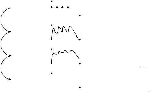
Figure 1. This figure briefly summarizes the functional pathways that exist from dosing (exposure) to outcome through drug biodistribution (pharmacokinetics) and drug effect (pharmacodynamics). it is not unusual to find a disconnect between the resolution available in the dynamic measurements and the actual clinical outcome. Also, while the convolution operator can be used to map the dosing regimen d(t) to the concentration-time profile c(t) and then to the effect e(t), this is not necessarily true when going from the dynamic behavior to clinical measurements, which are often lower resolution and/or discrete.
through sophisticated methodological contributions that have yet to impact the engineering mainstream. Lastly, the PK-PD model is currently viewed as a perfectly adequate approach not only to process, but to extract new, quantitative information from noisy measurements. As such, the model can be construed as a probe, or a measurement tool or medical instrument in its own right, with its own built-in confidence limits and design limitations (5).
Pharmacokinetics: What Shapes the Concentration–Time
Curve?
The first application of mathematical models to biology is usually attributed to Teorell (6) and led to the development of the class of compartmental models whose usage is now so widespread. Teorell’s work was conducted on exogenous substances, xenobiotics (e.g., drugs). Modelbased analysis of exogenous substances is somewhat simpler than endogenous compounds (e.g., glucose, insulin and other hormones, where autoregulation is crucial to understanding), since endogenous fluxes that may be exquisitely sensitive to changes in circulating concentrations are absent.
Teorell’s original motivation survives in modern PK-PD modeling. The PK model is typically a useful mathematical simplification of the underlying physicochemical and physiological processes. It is usually a lumped parameter, compartmental model, and describes the absorption, distribution, metabolism, and elimination (ADME) of a drug from the body (7). A practical review of simple PK models can be found, for example, in Ref. 8. As an example, the distribution of a drug in the plasma space following an intravenous injection may be well described by a monoexponential decay:
cðtÞ ¼ C0e at |
(1) |
where c(t) is the drug concentration at time t, C0 is the concentration at time 0 and a is the decay rate. As it is straightforward to verify, this functional form of c(t) is the solution to a first-order ordinary linear differential equation, or a single compartment model:
|
|
|
|
qðtÞ ¼ kelqðtÞ þ DdðtÞ |
|
||
qð0Þ ¼ |
0 |
(2) |
|
c t |
Þ ¼ |
qðtÞ |
|
ð |
V |
|
|
where q(t) is the amount of drug in the plasma space, D is the injected dose, d(t) is the Dirac delta, and V is the drug’s volume of distribution. It can be easily verified that
D C0 ¼ V
a ¼ kel
so that the elimination rate of the drug is equal to the decay rate of the concentration–time curve. An important pharmacokinetic parameter is the drug’s clearance, or the volume cleared per unit time, which for the model above can be expressed as:
CL ¼ kelV

Another common pharmacokinetic parameter is the area under the concentration curve:
Z
1
AUC ¼ cðtÞdt ¼ CLD
0
The AUC is probably the most common measure of exposure in pharmacokinetics, since it summarizes dosing and systematic information. The model in equation 2 could be extended to accommodate first-order absorption, for example, to model the plasma appearance of an oral or intramuscular dose as opposed to an intravenous dose:
|
ðtÞ ¼ kaq1 |
ðtÞ þ DdðtÞ |
|||
q1 |
|||||
|
ðtÞ ¼ þkaq1 |
ðtÞ kelq2 |
ðtÞ |
||
q2 |
|||||
q1ð0Þ ¼ q2ð0Þ ¼ 0 |
ð3Þ |
||||
c t |
Þ ¼ |
q2ðtÞ |
|
|
|
|
ð |
V |
|
|
|
where ka is the absorption rate constant (again in units of inverse time), and q1(t) and q2(t) are the amounts in the absorption compartment and in the plasma compartment, respectively. It can be easily verified that this model also describes the convolution of a single-exponential absorption forcing function with the single exponential impulse response of the plasma space.
For the simple single compartmental model (eq. 2), the pharmacokinetic parameters can be readily estimated from the data (9), and the assumption of a mechanistic model does not affect their values. In other words, both compartmental (model-dependent) and noncompartmental (datadependent) analyses provide the same result. However, this relatively straightforward interpretation of the eigenvalues of the system matrix in relation to the observed rate of decay is correct only for single-compartment systems such as this one. In the case when the drug diffuses in two compartments (e.g., a plasma and extravascular compartment), then its time course is described by a sum of two
exponential functions: |
|
cðtÞ ¼ A1e at þ A2e bt |
(4) |
but the corresponding ordinary linear differential equation is
q1ðtÞ ¼ ðk10 þ k12Þq1ðtÞ þ k21q2ðtÞ þ DdðtÞ
q2ðtÞ ¼ þk12q1ðtÞ k21q2ðtÞ
q1ð0Þ ¼ q2ð0Þ ¼ 0 |
(5) |
|
cðtÞ ¼ q1ðtÞ V
where the parameters are the same as before, except that now q1(t) and q2(t) are the amount of drug in the plasma and extraplasma compartments, respectively, k10 is the rate constant (in units of inverse time) at which the drug leaves the system, and k12 and k21 are the rate constants at which the drug is transported out of the plasma and extraplasma compartments, respectively. One can relatively easily estimate the a and b parameters describing the observed rates of decay (one slow and the other fast) of concentration; however, the algebraic relationship
PHARMACOKINETICS AND PHARMACODYNAMICS |
271 |
between those and the fractional rate constants that mechanistically describe plasma-extraplasma exchange is not trivial. The complexity of these expressions increases with increasing number of compartments (10) and rapidly grows to be daunting. The limitations of noncompartmental and compartmental analysis of pharmacokinetic data have been discussed elsewhere, so we will not cover them here (20). There are other sources of complexity in pharmacokinetics and drug metabolism, which turn into more complex expressions for the model equations required to describe the drug’s fate. For example, the underlying compartmental model may be not linear in the kinetics. This could happen, for example, when the fractional rate of disappearance changes with the drug level and goes from zero order at high concentrations to first order at low concentrations, as it happens for phenytoin (11) or ethanol (12):
|
|
|
|
Vm |
|
||
qðtÞ ¼ |
Km þ qðtÞ |
qðtÞ þ DdðtÞ |
(6) |
||||
qð0Þ ¼ 0 |
|||||||
|
|||||||
c t |
Þ ¼ |
qðtÞ |
|
|
|||
ð |
V |
|
|||||
where the elimination rate is not constant, rather it exhibits a saturative behavior that resembles the classic Michaelis–Menten expression from enzyme kinetics. In this case, the principle of superposition does not hold and the concentration–time curve cannot be expressed in algebraic (closed) form, and the time course is not exponential, except at values of q(t) that are much smaller than Km. There are many other types of pharmacokinetic nonlinearities, of which this is just an example. This is why most modern PK analyses directly use the differential equations when building a PK model.
Excellent historical reviews of the properties of compartmental models, especially with reference to tracer kinetics, can be found in Refs. 13–16. More modern viewpoints are available in Refs. 17,18. Perspectives from drug development are available in Refs. 7,19. A succinct and practical review of compartmental and noncompartmental methods can be found in Ref. 8. Lastly, as we mentioned, a comparison of the strengths and weaknesses of compartmental and noncompartmental approaches has been carried out in Ref. 20.
A PK model can be used to make informed predictions about localized drug distribution and dose availability to the target organ, especially with physiologically based pharmacokinetic (PBPK) and toxicokinetic (PBTK) models. An important application has always been to individualize dosing (21,22) and improve therapeutic drug monitoring (23,24), often by borrowing approaches from process engineering and automatic control theory (25,26). Physiologically based models of pharmacokinetics are becoming an integral part of many drug development programs (27), mainly because they provide a mechanistic way to scale dosing regimens between species and between protocols. This affords (at least in theory) a seamless integration between the preclinical (in vitro and in vivo, animal studies) and clinical (in vivo, human studies) aspects of a drug development program. Animal to human scaling is of

272 PHARMACOKINETICS AND PHARMACODYNAMICS
increasing importance in several areas of pharmacotherapy (28) and has a long and illustrious history, from the early work by Dedrick and co-workers on methotrexate (29) to a more general application (30,31) to modern experiences (32) motivated by first time in man (FTIM) dose finding (33,34). The approach is, however, not without its critics (35), mainly due to the lack of statistical evaluation that often accompanies the scaling. It is noteworthy that between-species scaling of body mass (36,37) and metabolic rate (38) has been and is currently an object of investigation outside drug development, and mechanistic findings about the origin of allometric scaling (39) have lent scientific support to the empiricism of techniques used in drug development (40,41).
Now is a good time to note that, most often, these projections are accompanied by some statistical evaluation. From the very beginnings of PK-PD, the realization that one needed to account both for variation between subjects (due to underlying biological reasons, e.g., genetic polymorphisms and environmental factors) and variation within subject (due, e.g., to intrinsic measurement error associated with the quantification of concentration time courses and efficacy levels) was particularly acute. Statistical considerations have thus always been a part of PKPD. The role of population analysis, or the explicit modeling of variability sources, in the analysis of clinical trial data is discussed in more detail later. As far as other examples, statistical applications to PK-PD have proven useful in aiding the estimation of rates of disease progression (42,43), determining individually tailored dosing schemes (23,44) and resolving models too complex to identify without prior information (45). As mentioned later, a common framework often exploited in PK-PD has to do with the incorporation of population-level information (e.g., statistical distributions of model parameters) together with individual-specific information (limited concentration–time samples, e.g.).
Pharmacodynamics: The Mechanistic Link Between Drug
Exposure and Effect
The PD models (46–49) can link drug effect (characterized by clinical outcomes or intermediate pharmacological response markers) with a PK model (50), through biophase distribution, biosensor process and biosignal flux (51). Formally, the simplest PD model is the so-called Emax model, where effect plateaus at high concentrations:
e t |
Þ ¼ |
EmaxcðtÞ |
(7) |
ð |
EC50 þ cðtÞ |
|
where Emax is maximal effect, and EC50 is the effective plasma concentration at which effect e(t) is half-maximal. This model is sometimes modified to account for sigmoidal effect shapes by adding an exponent that varies from 1 to around 2:
e t |
Þ ¼ |
EmaxcHðtÞ |
(8) |
|
EC50H þ cHðtÞ |
||||
ð |
|
Often, the driver of pharmacological effect is not plasma concentration c(t), but some concentration remote from plasma and delayed with respect to plasma. This repre-
sentation is similar to the one used to represent delayed effect of glucose regulatory hormones such as insulin (52). The delayed effect site concentration is them modeled using the differential equation:
ceðtÞ ¼ keo½cðtÞ ceðtÞ& |
(9) |
whereas the PD model now contains effect site concentration, not plasma concentration:
e t |
Þ ¼ |
EmaxceðtÞ |
(10) |
ð |
EC50 þ ceðtÞ |
|
and the interpretation of the parameters is the same as before except that they are defined with reference to effect site concentration as opposed to plasma concentration. Other classes of models are the so-called indirect response models, where the drug modulates either production or degradation of the effect (response) variable. These models are particularly appealing due to their mechanistic interpretation, and have been proposed in Refs. (53) and (54), reviewed in Ref. (55), and applied in many settings, including pharmacogenomics (56).
In many ways, the PD aspect of drug development is more challenging than the PK aspects, for many different reasons. First of all, the process of gathering data to inform about the PD of a drug is more challenging. Moreover, PD measurements may be less sensitive than it would be desirable (pain levels, which are both categorical and subjective, are a good example). Lastly, the mechanism of action of the drug may not be entirely known, and thus the best choice of measurements for the PD time course may be open to debate. How should the effect of a certain drug be quantified? If the drug is a painkiller, are pain levels sufficient, or would the levels of certain chemical(s) in the brain provide a more sensitive and specific correlate of efficacy? These and other questions become very relevant, for example, when drugs are studied that exert their effect in traditionally inaccessible locations (e.g., the brain) (57).
This is the ‘‘best biomarker question’’, as it relates to the now classical classification of biomarkers, surrogate endpoints and clinical endpoints (58). Basically, while a biomarker is any quantitative measure of a biological process (concentration levels, pain scores, test results and the like), a surrogate endpoint is a biomarker that substitutes for a clinical endpoint (e.g., survival or remission). In other words, surrogate endpoints, when unambiguously defined, are predictive of clinical endpoints, with the added advantage of being easier to measure and usually being characterized by a more favorable time frame (59). In the United States, the Food and Drug Administration (FDA) now allows the possibility of accelerated approval based on surrogate endpoints, provided certain conditions are met (60). Against this framework, it makes eminent sense for the PK-PD model to be focused on a relevant biomarker (or surrogate endpoint) as soon as possible in the drug development process. Often, the earlier in the process, the less influence the choice of biomarker will have. In other words, when the selection of lead compounds is just starting, proof of concept may be all that is needed, but the closer one gets to the clinical trial stage, the more crucial an appropriate

choice of surrogate endpoint will be. Another way to think about this is the establishment of a causal link between therapeutic regimen and outcome. Where these concepts come together is in the (relatively novel) idea of disease progression, and how it can be monitored.
Disease Progression: How to Know Whether the Drug is Working
Recently, the contention has been made that an integral part of the understanding of PK and PD cannot prescind from, say, the background signal that is present when the drug is administered. In other words, not all patients will be subjected to therapy at the same point in time, or at the same stage in their individual progression from early to late disease stages. There is thus a growing realization that the therapeutic intervention is made against a constantly changing background of disease state, and that the outcome of the therapy may depend on the particular disease state at a given moment in time. Disease progression modeling (61) is thus the point of contact between PK and PD and the mechanistic modeling of physiology and pathophysiology that is advocated, e.g., by the Physiome Project (62,63), recently taken over by the International Union of Physiological Sciences’ Physiome and Bioengineering Committee (64).
Interesting applications are starting to emerge. For example, Ref. 65 has shown that the rate of increase of bloodstream glucose concentration in Type 2 diabetic patients is 0.84 mmol L 1 year 1 (with a sizable variation between patients of 143%), thus providing a quantitative handle on the expected deteriorating trend of overall glycemic levels in this population of patients (together with a measure of its expected patient-to-patient variability). In Alzheimer’s disease, another study (66) has demonstrated a natural rate of disease progression of 6.17 ADASC units year 1 (where ADASC is the cognitive component of the Alzheimer disease assessment scale). A word of caution: As often done in this area of application, the models are informed on available data. In other words, the model parameters are quantified (estimated) based on available measurements for the drug PK and PD. This poses the challenge of developing models that are not too detailed nor too simplistic, but that can be reasonably well informed by the data at hand. Clearly, a detailed mechanistic model of the disease system requires substantial detail, but a balance needs to be struck between detail and availability of independently gathered data. Visualization approaches are a recent addition to the arsenal of the drug development expert (67). This kind of mechanistic pharmacodynamics is being applied more and more often to a variety of areas: A good example of rapid development comes from anticancer agents (68), where applications of integrated, mechanistic PK-PD models that take into account the drug mechanism of action are starting to become more and more frequent (69).
Population Variation: Adding Statistical Variation to PK, PD and Disease Models
In drug development, it is of utmost interest to determine the extent of variation of PK-PD and disease progression
PHARMACOKINETICS AND PHARMACODYNAMICS |
273 |
among members of a population. Basically, this implies determining the statistics of the biomarkers of interest in a population of patients, not just in an individual, and provide these measures together with some degree of confidence. This requirement connects well with analogous epidemiological population studies (often not modelbased). The estimation of variability coupled with the evaluation of the relative role of its sources (covariates), for example, demographics, anthropometric variables or genetic polymorphisms, is tackled by the discipline of population kinetics, mainly due to the pioneering work of Lewis Sheiner and Stuart Beal at UCSF (70,71). Often called also population PK-PD, it makes use of two-level hierarchical models characterized by nested variability sources, where the models’ individual parameter values are not deterministic, but unknown: They instead arise from population statistical distributions (biological variation, or BSV, between subject variability). On top of this source of variability, measurement noise and other uncertainty sources are added (RUV, residual unknown variation) to the concentration or effect signals (Fig. 2). The pharmaco-statistical models that integrate BSV and RUV are often described in statistical journals as nonlinear mixed effects models.
An example that builds on those we have already presented earlier may suffice here to clarify the fundamental concept of mixed effects models. Let us extend the model just described for intravenous injection (eq. 2) to the situation when the concentration measurements are affected by noise:
|
|
|
|
|
qðtÞ ¼ kelqðtÞ þ DdðtÞ |
||||
qð0Þ ¼ 0 |
|
(11) |
||
c t |
Þ ¼ |
qðtÞ |
t |
Þ |
ð |
V |
þeð |
||
where the parameters are the same as in equation 2, except that now e(t) is a normally distributed measurement error with mean zero and variance s2, that is e(t)2N[0, s2]. If data about c(t) are available and have been gathered in a single individual, the model parameters kel and V (assuming D is known) can then be fitted to the data using weighted (9) or extended (72) least squares or some other variation of maximum likelihood, and thus individualized estimates (with confidence intervals) can be obtained (often the measurement error variance s2 is not known but it can also be estimated). This can be done even if only a single subject data are available, provided that the sampling is performed (at an absolute minimum) at three or more time points (since the model has two unknown structural parameters, kel and V, plus s2).
The nonlinear mixed-effects modeling approach is an extension of what we have just seen. It takes the viewpoint that the single subject estimates are realizations of an underlying population density for the model parameters. As such, the individual values of kel and V simply become realizations (samples) of this underlying density. For example, the assumption could be made that they are both distributed lognormally: in which case, log(kel)2N(mkel,
v2kel) and log(V)2N(mn, v2n), where the m denote expected logarithmic values and the v2 denote population variances.
274 PHARMACOKINETICS AND PHARMACODYNAMICS
units) |
12.00 |
|
|
|
|
|
12.00 |
|
|
|
|
|
|
|
|
|
|
|
|
A |
|
|
|
|
|
|
|
B |
|
10.00 |
|
|
|
|
|
10.00 |
|
|
|
|
|
|
||
(arbitrary |
|
|
|
|
|
|
|
|
|
|
|
|||
8.00 |
|
|
|
|
|
|
8.00 |
|
|
|
|
|
|
|
|
|
|
|
|
|
|
|
|
|
|
|
|
|
|
Drug Concentration |
6.00 |
|
|
|
|
|
|
6.00 |
|
|
|
|
|
|
4.00 |
|
|
|
|
|
|
4.00 |
|
|
|
|
|
|
|
2.00 |
|
|
|
|
|
|
2.00 |
|
|
|
|
|
|
|
0.00 |
|
|
|
|
|
|
0.00 |
|
|
|
|
|
|
|
|
0.00 |
4.00 |
8.00 |
12.00 |
16.00 |
20.00 |
24.00 |
0.00 |
4.00 |
8.00 |
12.00 |
16.00 |
20.00 |
24.00 |
units) |
12.00 |
|
|
|
|
|
12.00 |
|
|
|
|
|
|
|
|
|
|
|
|
C |
|
|
|
|
|
|
|
D |
|
10.00 |
|
|
|
|
|
10.00 |
|
|
|
|
|
|
||
(arbitrary |
|
|
|
|
|
|
|
|
|
|
|
|||
8.00 |
|
|
|
|
|
8.00 |
|
|
|
|
|
|
||
|
|
|
|
|
|
|
|
|
|
|
|
|
|
|
Concentration |
6.00 |
|
|
|
|
|
6.00 |
|
|
|
|
|
|
|
4.00 |
|
|
|
|
|
4.00 |
|
|
|
|
|
|
||
2.00 |
|
|
|
|
|
2.00 |
|
|
|
|
|
|
||
Drug |
|
|
|
|
|
|
|
|
|
|
|
|||
0.00 |
|
|
|
|
|
0.00 |
|
|
|
|
|
|
||
|
|
|
|
|
|
|
|
|
|
|
|
|||
|
0.00 |
4.00 |
8.00 |
12.00 |
16.00 |
20.00 |
24.00 |
0.00 |
4.00 |
8.00 |
12.00 |
16.00 |
20.00 |
24.00 |
Time (arbitrary units) |
Time (arbitrary units) |
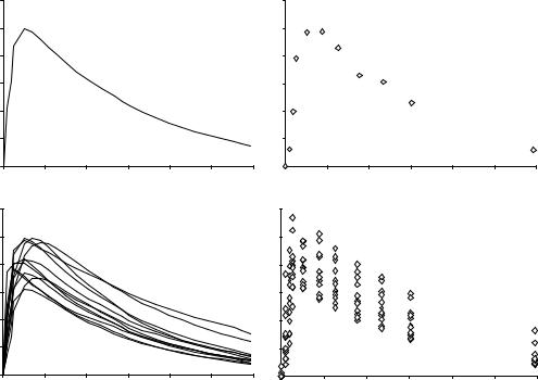
Figure 2. Nested uncertainty in pharmacokinetics. Panel A shows the true, but unknown, time course over 24 time units of a hypothetical drug administered orally to a single experimental subject. The true, but unknown, time course is a smooth function of time. Panel B shows the same smooth function sampled at discrete time points, which in practice may correspond to as many blood draws. Measurement uncertainty (currently termed RUV, residual unknown variability) is now superimposed to the true, but unknown time course in Panel A. Panel C shows the true, but unknown, time course over 24 time units of a hypothetical drug administered orally to several experimental subjects. Clearly, no time course is the same, since each subject will have a different absorption and elimination rate, together with a different volume of distribution. The time courses in Panel C are the result of BSV (between subject variability). Lastly, Panel D shows the same smooth functions in Panel c sampled at discrete time points. The RUV is again superimposed to the true, but unknown time courses, but this time the data spread is due to both BSV and RUV, and distinguishing between BSV and RUV requires a model of the system. See text for details.
The assumption is implicitly made here that kel and V are uncorrelated (which may or may not be the case). In the nonlinear mixed-effects model procedure, the moments of the statistical distributions of model parameters become
the new unknowns, and thus mk01, v2k01 and mn, v2n are estimated by optimizing approximations of the maxi-
mum likelihood objective function expressed for the whole population of data. The value of s2 in the population (a composite value of the measurement error variance across subjects) can also be estimated, as before. The five distribution parameters are the fixed effects of the population (since they do not change between subject), while the individual values attained by the parameters kel and V in separate individuals are random effects, since every subject has a different value (hence, the mixed-effects parlance). The approach requires data on more than one subject, ideally on many more subjects than there are fixed effects (the caveat is that it is easier to estimate expected values than it is to estimate variances or covariances, and the data needs consequently grow). Note also
that, if kel and V are both lognormal, clearance CL is not lognormal: which statistical model to choose for which parameter will depend on the available information. The main advantage of population kinetics is that, since it is estimating distributional parameters (moments), it can use relatively sparse and/or noisy data at the individual level, provided that there is a large number of population data (in other words, there can be few data for each subject, as long as there are many subjects).
This framework is quite general and powerful, and allows for modeling of complex events (e.g., adherence, or patient compliance to dosing recommendations) (73). Tutorials on this modeling approach can be found in papers (74–76), review articles (70,61,77,78), and textbooks (79). Software is also available, both for population (Aarons, 1999) and individual (Charles and Duffull, 2001) PK-PD analysis.
Mixed-effects models are used both to solve the forward problem (simulation of putative drug dosing scenarios) and the inverse problem (estimation of BSV and RUV statistics conditional on PK-PD models and clinical
measurements). Which one is of interest depends on what is available and what the intent of the study is. If the intent is to analyze data and determine the underlying distribution of PK-PD and disease parameters, then one has an inverse, or estimation, problem (80). If the intent, on the other hand, is to explore possible dosing or recruitment scenarios, then this is a direct, or simulation, problem (81). As mentioned, mixed-effects models can be applied to sparse and noisy data, as often happens in therapeutic monitoring in the clinical setting (a situation that occurs both in drug development and in applied clinical research). Their use is so widespread that the FDA recently issued one of its guidances for industry to deal with their use for population pharmacokinetic analysis (82). Interestingly, a very similar framework is also applied to evolutionary genetics, in the study of ‘‘function-valued traits’’ (also called ‘‘infinite-dimensional characters’’). The idea is to use mixed models to link genetic information to traits that are not constant, rather are functions of time (83–85). It is important to model population genetics both for polymorphisms of drug-metabolizing enzymes affecting ADME and for polymorphisms affecting the dynamics of response.
A Role for Modeling and Simulation
In summary, the overall goal of integrated PK-PD mathematical models is a better understanding of therapeutic intervention: Their contribution are often reflected in improved clinical trials designs. While evidence of the impact of modeling and simulation of PK-PD on the drug development process is often anectodal, many reviews of PK-PD in drug development have recently appeared (86–89), together with compelling examples of subsequent drug development acceleration (90,91).
While the fundamental algorithmic steps of computer simulation, especially Monte Carlo simulation, are well known, they require some adaptation to be used within the field of pharmacokinetics and pharmacodynamics and in the context of drug development (Fig. 3) A good practices document was issued in 1999 following a workshop held by the Center for Drug Development Science (92). The crafting of this document has contributed to clarifying the steps and tools necessary for carrying out a simulation experiment within the context of drug development. In particular, the report clarifies that simulation in drug development has an untapped potential which extends well beyond the pharmacokinetic aspect and into the pharmacodynamic and clinical domains (92).
Nowadays, pharmacometric technology (93) is used in industry and academia as a way to support and strengthen R&D. As an example, low signal/noise ratio routine clinical data obtained with sparse sampling may often be analyzed with pharmacometric techniques to determine whether a compound is metabolized differently because of phenotypic differences arising from genetic makeup, ethnicity, gender, age group (young, elderly), or concomitant medications causing drug–drug interactions (94). The role of this technology can only increase. A recently issued FDA report that focuses on the recent decrease in applications for novel therapies submitted to the agency is clear in this regard: ‘‘The concept of model-based drug development, in which
PHARMACOKINETICS AND PHARMACODYNAMICS |
275 |
|||
Dosing |
Measured |
Drug |
Data |
|
regimen |
concentration |
effect |
|
|
|
|
|||
PK |
Disease |
PD |
Models |
|
model |
model |
model |
|
|
|
|
|||
Estimation of system parameters
Simulations of trial scenarios Findings Simulations of disease progress
Simulations of dosage regimens and treatment effects
Figure 3. Information flow in a clinical trial simulation or data analysis. The doses, the measured concentration and drug effect are situated at the beginning or the end of the process (Data level). At the core of the simulation (Model level) lie models of PK, PD and disease processes. Trial designs are possible conditional on these other elements, or features like model parameters can be estimated from the trial data and measured doses and PK and PD data (Findings level). The picture is oversimplified and does not include, for example, adherence to dosing recommendations and protocol dropouts, which may be important to ensure realistic trial designs.
pharmaco-statistical models of drug efficacy and safety are developed from preclinical and available clinical data, offers an important approach to improving drug development knowledge management and development decision making. Model-based drug development involves building mathematical and statistical characterizations of the time course of the disease and drug using available clinical data to design and validate the model. The relationship between drug dose, plasma concentration, biophase concentration (pharmacokinetics), and drug effect or sideeffects (pharmacodynamics) is characterized, and relevant patient covariates are included in the model. Systematic application of this concept to drug development has the potential to significantly improve it’’ (95).
In summary, modern-day drug development displays a need for information integration at the whole-system, cellular, and genomic level (96) similar to that found in integrative physiology (97) and comparative biology (98,99). As mentioned earlier, simulation of clinical trials is a burgeoning discipline well-founded upon engineering and statistics (81): examples have appeared in clinical pharmacology (100,101) and pharmacoeconomics (102). Drug candidate selection is another application, possibly through PK models of varying complexity (103) and high throughput screening coupled with PK (104). Next, integrated models allow to link genomic information with disease biomarkers and phenotypes, such as in the LuoRudy model of cardiac excitation (105).
As a concluding remark, progress in the development of plausible, successful, and powerful data analysis methods has already had a substantial payoff, and can be substantially accelerated by encouraging multidisciplinary, multiinstitutional collaboration bringing together investigators at multiple facilities and providing the infrastructure to support their research, thus allowing the timely and costeffective expansion of new technologies. The need is more
276 PHARMACOKINETICS AND PHARMACODYNAMICS
and more often voiced for increased training of quantitative scientists in biologic research as well as in statistical methods and modeling to ensure that there will be an adequate workforce to meet future research needs (106).
BIBLIOGRAPHY
1.Marasco C. Surge In Pharmacometrics Demand Leads to New Master’s Program. JobSpectrum.org – a service of the American Chemical Society. Available at http://www. cen-chemjobs.org/job_weekly31802.html, 2002.
2.Abdel-Rahman SM Kauffman RE. The integration of pharmacokinetics and pharmacodynamics: understanding doseresponse. Annu Rev Pharmacol Toxicol 2004;44:111–136.
3.Rowland M, Tozer TN. Clinical Pharmacokinetics: Concepts and Applications. 3rd Ed. Baltimore: Williams & Wilkins; 1995.
4.Verotta D. Volterra series in pharmacokinetics and pharmacodynamics. J Pharmacokinet Pharmacodyn. 2003;30(5): 337–362.
5.Vicini P, Gastonguay MR, Foster DM. Model-based approaches to biomarker discovery and evaluation: a multidisciplinary integrated review. Crit Rev Biomed Eng 2002;30 (4–6):379–418.
6.Teorell T. Kinetics of distribution of substances administered to the body. I. The extravascular modes of administration. II. The intravascular modes of administration. Arch Int Pharmacodyn Ther. 1937; 57: 205–240.
7.Gibaldi M, Perrier D. Pharmacokinetics, 2nd Ed. New York: Marcel Dekker; 1982.
8.Jang GR, Harris RZ, Lau DT. Pharmacokinetics and its role in small molecule drug discovery research. Med Res Rev 2001;21(5):382–396.
9.Landaw EM, DiStefano JJ 3rd. Multiexponential, multicompartmental, and noncompartmental modeling. II. Data analysis and statistical considerations. Am J Physiol 1984;246(5 Pt. 2):R665–77.
10.DiStefano JJ 3rd, Landaw EM. Multiexponential, multicompartmental, and noncompartmental modeling. I. Methodological limitations and physiological interpretations. Am J Physiol 1984;246(5 Pt. 2):R651–664.
11.Grasela TH, et al. Steady-state pharmacokinetics of phenytoin from routinely collected patient data. Clin Pharmacokinet 1983;8(4):355–364.
12.Holford NH. Clinical pharmacokinetics of ethanol. Clin Pharmacokinet, 1987;13(5):273–292.
13.Anderson DH. Compartmental Modeling and Tracer Kinetics. Lecture Notes in Biomathematics, Vol. 50, Berlin: SpringerVerlag; 1983.
14.Godfrey K. Compartmental Models and Their Application. New York: Academic; 1983.
15.Jacquez JA. Compartmental Analysis in Biology and Medicine, 2nd ed. Michigan: University of Michigan Press; 1985.
16.Carson ER, Cobelli C, Finkelstein L. The Mathematical Modeling of Endocrine-Metabolic Systems. Model Formulation, Identification and Validation. New York: Wiley; 1983.
17.Carson E, Cobelli C. Modelling Methodology for Physiology and Medicine. San Diego: Academic Press; 2000.
18.Cobelli C, Foster D, Toffolo G. Tracer Kinetics in Biomedical Research: From Data to Model. London: Kluwer Academic/ Plenum; 2001.
19.Atkinson AJ, et al., eds. Principles of Clinical Pharmacology. San Diego: Academic Press; 2001.
20.DiStefano JJ 3rd. Noncompartmental vs. compartmental analysis: some bases for choice. Am J Physiol 1982;243(1): R1–6.
21.Goicoechea FJ, Jelliffe RW. Computerized dosage regimens for highly toxic drugs. Am J Hosp Pharm 1974;31(1):67–71.
22.Sheiner LB, Beal S, Rosenberg B, Marathe VV. Forecasting individual pharmacokinetics. Clin Pharmacol Ther 1979;26(3):294–305.
23.(a) Jelliffe RW, et al. Individualizing drug dosage regimens: roles of population pharmacokinetic and dynamic models, Bayesian fitting, and adaptive control. Ther Drug Monit 1993;15(5):380–393. (b) Jelliffe RW. Clinical applications of pharmacokinetics and adaptive control. IEEE Trans Biomed Eng 1987;34(8):624–632.
24.(a) Jelliffe RW, et al. Adaptive control of drug dosage regimens: basic foundations, relevant issues, and clinical examples. Int J Biomed Comput 1994;36(1–2):1–23. (b) Jelliffe RW, Schumitzky A. Modeling, adaptive control, and optimal drug therapy. Med Prog Technol 1990;16(1–2):95–110.
25.Jelliffe RW. Clinical applications of pharmacokinetics and adaptive control. IEEE Trans Biomed Eng 1987;34(8):624– 632.
26.Jelliffe RW, Schumitzky A. Modeling, adaptive control, and optimal drug therapy. Med Prog Technol 1990;16(1–2):95–110.
27.Parrott N, Jones H, Paquereau N, Lave T. Application of full physiological models for pharmaceutical drug candidate selection and extrapolation of pharmacokinetics to man. Basic Clin Pharmacol Toxicol 2005;96(3):193–199.
28.Gallo JM, et al. Pharmacokinetic model-predicted anticancer drug concentrations in human tumors. Clin Cancer Res 2004;10(23):8048–8058.
29.Dedrick R, Bischoff KB, Zaharko DS. Interspecies correlation of plasma concentration history of methotrexate (NSC-740). Cancer Chemother Rep 1970;54(2):95–101.
30.Dedrick RL. Animal scale-up. J Pharmacokinet Biopharm 1973;1(5):435–461.
31.Dedrick RL, Bischoff KB. Species similarities in pharmacokinetics. Fed Proc 1980;39(1):54–59.
32.Mahmood I, Balian JD. Interspecies scaling: predicting clearance of drugs in humans. Three different approaches. Xenobiotica 1996;26(9):887–895.
33.Mahmood I, Green MD, Fisher JE. Selection of the first-time dose in humans: comparison of different approaches based on interspecies scaling of clearance. J Clin Pharmacol 2003;43(7):692–697.
34.Iavarone L, et al. First time in human for GV196771: interspecies scaling applied on dose selection. J Clin Pharmacol 1999;39(6):560–566.
35.Bonate PL, Howard D. Prospective allometric scaling: does the emperor have clothes? J Clin Pharmacol 2000;40(6):665–670. discussion 671–676.
36.West GB, Brown JH, Enquist BJ. A general model for the origin of allometric scaling laws in biology. Science 1997;276(5309):122–126.
37.(a) Iavarone L, et al. First time in human for GV196771: interspecies scaling applied on dose selection. J Clin Pharmacol 1999;39(6):560–566. (b) West GB, Brown JH, Enquist BJ. The fourth dimension of life: fractal geometry and allometric scaling of organisms. Science 1999;284(5420):1677– 1679.
38.Gillooly JF, et al. Effects of size and temperature on metabolic rate. Science 2001;293(5538):2248–2251. Erratum in Science 2001;294(5546):1463.
39.White CR, Seymour RS. Mammalian basal metabolic rate is proportional to body mass2/3. Proc Natl Acad Sci USA 2003;100(7):4046–4049.
40.Anderson BJ, Woollard GA, Holford NH. A model for size and age changes in the pharmacokinetics of paracetamol in neonates, infants and children. Br J Clin Pharmacol 2000;50(2): 125–134.
41.van der Marel CD, et al. Paracetamol and metabolite pharmacokinetics in infants. Eur J Clin Pharmacol 2003;59(3): 243–251.
42.Craig BA, Fryback DG, Klein R, Klein BE. A Bayesian approach to modelling the natural history of a chronic condition from observations with intervention. Stat Med 1999;18(11):1355– 1371.
43.Mc Neil AJ. Bayes estimates for immunological progression rates in HIV disease. Stat Med 1997;16(22):2555–2572.
44.Sheiner LB, Beal SL. Bayesian individualization of pharmacokinetics: simple implementation and comparison with non-
Bayesian methods. J Pharm Sci 1982;71(12):1344– 1348.
45.Cobelli C, Caumo A, Omenetto M. Minimal model SG overestimation and SI underestimation: improved accuracy by a Bayesian two-compartment model. Am J Physiol 1999;277 (3 Pt.1):E481–488.
46.Segre G. Kinetics of interaction between drugs and biological systems. Farmaco [Sci] 1968;23(10):907–918.
47.Dahlstrom BE, Paalzow LK, Segre G, Agren AJ. Relation between morphine pharmacokinetics and analgesia. J Pharmacokinet Biopharm 1978 6(1):41–53.
48.Holford NH, Sheiner LB. Pharmacokinetic and pharmacodynamic modeling in vivo. CRC Crit Rev Bioeng 1981a;5(4): 273–322.
49.Holford NH, Sheiner LB. Understanding the dose-effect relationship: clinical application of pharmacokineticpharmacodynamic models. Clin Pharmacokinet 1981b; 6(6):429–453.
50.Holford NH, Sheiner LB. Kinetics of pharmacologic response. Pharmacol Ther 1982;16(2):143–166.
51.Jusko WJ. Pharmacokinetics and receptor-mediated pharmacodynamics of corticosteroids. Toxicology 1995;102(1–2): 189–196.
52.Bergman RN, Phillips LS, Cobelli C. Physiologic evaluation of factors controlling glucose tolerance in man: measurement of insulin sensitivity and beta-cell glucose sensitivity from the response to intravenous glucose. J Clin Invest 1981;68(6): 1456–1467.
53.(a) Dayneka NL, Garg V, Jusko WJ. Comparison of four basic models of indirect pharmacodynamic responses. J Pharmacokinet Biopharm 1993;21(4):457–478. (b) Ramakrishnan R, et al. Pharmacodynamics and pharmacogenomics of methylprednisolone during 7-day infusions in rats. J Pharmacol Exp Ther 2002;300(1):245–256.
54.Jusko WJ, Ko HC. Physiologic indirect response models characterize diverse types of pharmacodynamic effects. Clin Pharmacol Ther 1994;56(4):406–419.
55.Sharma A, Jusko WJ. Characteristics of indirect pharmacodynamic models and applications to clinical drug responses. Br J Clin Pharmacol 1998;45(3):229–239.
56.Ramakrishnan R, et al. Pharmacodynamics and pharmacogenomics of methylprednisolone during 7-day infusions in rats.J Pharmacol Exp Ther 2002;300(1):245–256.
57.Bieck PR, Potter WZ. Biomarkers in psychotropic drug development: integration of data across multiple domains. Annu Rev Pharmacol Toxicol 2005;45:227–246.
58.Biomarkers Definitions Working Group. Biomarkers and surrogate endpoints: preferred definitions and conceptual framework. Clin Pharmacol Ther 2001;69(3):89–95.
59.Rolan P, Atkinson AJ Jr., Lesko LJ. Use of biomarkers from drug discovery through clinical practice: report of the Ninth European Federation of Pharmaceutical Sciences Conference on Optimizing Drug Development. Clin Pharmacol Ther 2003;73(4):284–291.
60.The Food and Drug Modernization Act of 1997. Title 21 Code of Federal Regulations Part 314 Subpart H Section 314.500.
PHARMACOKINETICS AND PHARMACODYNAMICS |
277 |
61.Chan PL, Holford NH. Drug treatment effects on disease progression. Annu Rev Pharmacol Toxicol 2001;41:625–659.
62.Bassingthwaighte JB. The macro-ethics of genomics to health: the physiome project. C R Biol 2003;326(10–11): 1105–1110.
63.Hunter PJ, Borg TK. Integration from proteins to organs: the Physiome Project. Nat Rev Mol Cell Biol 2003;4(3):237– 243.
64.Hunter PJ. The IUPS Physiome Project: a framework for computational physiology. Prog Biophys Mol Biol 2004; 85(2–3):551–569.
65.Frey N, et al. Population PKPD modelling of the long-term hypoglycaemic effect of gliclazide given as a once-a-day modified release (MR) formulation. Br J Clin Pharmacol 2003;55(2):147–157.
66.Holford NH, Peace KE. Methodologic aspects of a population pharmacodynamic model for cognitive effects in Alzheimer patients treated with tacrine. Proc Natl Acad Sci USA 1992;89(23):11466–11470.
67.Bhasi K, Zhang L, Zhang A, Ramanathan M. Analysis of pharmacokinetics, pharmacodynamics, and pharmacogenomics data sets using VizStruct, a novel multidimensional
visualization technique. Pharm Res 2004;21(5):777– 780.
68.Friberg LE, Karlsson MO. Mechanistic models for myelosuppression. Invest New Drugs 2003;21(2):183–194.
69.Karlsson MO, et al. Pharmacokinetic/pharmacodynamic modelling in oncological drug development. Basic Clin Pharmacol Toxicol 2005;96(3):206–211.
70.Beal SL, Sheiner LB. Estimating population kinetics. Crit Rev Biomed Eng 1982;8(3):195–222.
71.Sheiner LB, Ludden TM. Population pharmacokinetics/ dynamics. Annu Rev Pharmacol Toxicol 1992;32:185– 209.
72.Peck CC, Beal SL, Sheiner LB, Nichols AI. Extended least squares nonlinear regression: a possible solution to the ‘choice of weights’’ problem in analysis of individual pharmacokinetic data. J Pharmacokinet Biopharm 1984;12(5): 545– 558.
73.Girard P, et al. A Markov mixed effect regression model for drug compliance. Stat Med 1998;17(20):2313–2333.
74.Sheiner LB. Analysis of pharmacokinetic data using parametric models-1: Regression models. J Pharmacokinet Biopharm 1984;12(1):93–117.
75.(a) Landaw EM, DiStefano JJ 3rd. Multiexponential, multicompartmental, and noncompartmental modeling. II. Data analysis and statistical considerations. Am J Physiol 1984; 246(5 Pt. 2):R665–77. (b) Sheiner LB. Analysis of pharmacokinetic data using parametric models. II. Point estimates of an individual’s parameters. J Pharmacokinet Biopharm 1985; 13(5):515–540.
76.Sheiner LB. Analysis of pharmacokinetic data using parametric models. III. Hypothesis tests and confidence intervals. J Pharmacokinet Biopharm 1986;14(5):539–555.
77.Ette EI, Williams PJ. Population pharmacokinetics II: estimation methods. Ann Pharmacother 2004;38(11):1907–1915.
78.Ette EI, Williams PJ. Population pharmacokinetics I: background, concepts, and models. Ann Pharmacother 2004; 38(10):1702–1706.
79.Davidian M,and Giltinan DM. Nonlinear Models for Repeated Measurement Data. Boca Raton: Chapman and Hall/CRC; 1995.
80.Sheiner L, Wakefield J. Population modelling in drug development. Stat Methods Med Res 1999;8(3):183–193.
81.Holford NH, Kimko HC, Monteleone JP, Peck CC. Simulation of clinical trials. Annu Rev Pharmacol Toxicol 2000;40:209– 234.