

106 NUCLEAR MEDICINE, COMPUTERS IN
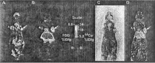
Figure 17. A PET animal scanner murine image. Both FDG (Image a) and 64Cu-minibody (Image b) were used as radiotracers. Images c and d show pathology and autoradiographic results, respectively.
assays. As mentioned there remains the difficulty of finding a suitable positron emitter and method of attachment for a particular imaging experiment.
Hybrid Animal Imaging Devices
Quantitation of radioactivity at sites within the mouse’s body is more easily done with an animal gamma camera than in the comparable clinical situation. This follows since attenuation of photons is relatively slight for a creature only a few cm thick in most cross-sections. Because of this simplicity, the output of the small animal gamma camera imaging systems can be modified to yield percent-injected dose (%ID). In order to correct for organ perfusion, it is historically conventional in biodistribution work using sacrificed animals to obtain uptake in %ID/g of tissue. Given the organ %ID, this last parameter may be obtained if the total mass of the target organ can be determined. Two avenues are available; one may employ miniaturized CT or a reference table of organ sizes for the particular strain of animal being imaged. We should note that suitably sized CT scanners are produced commercially and may be used to estimate organ mass. Hybrid SPECT/CT, PET–CT and SPECT–PET–CT animal imagers are now available for mouse-sized test animals.
One caveat regarding the small-scale imaging devices should be added; these systems cannot give entirely comparable results to biodistribution experiments. In animal sacrifice techniques, essentially any tissue may be dissected for radioactivity assay in a well counter. Miniature cameras and PET systems will show preferentially the highest regions of tracer accumulation. Many tissues may not be observable as their activity levels are not above blood pool or other background levels. Hybrid animal scanners can reduce this limitation, but not eliminate it entirely. Those developing new pharmaceuticals may not be concerned about marginal tissues showing relatively low accumulation, but regulatory bodies, such as the U.S. Food and Drug Administration (FDA), may require their measurement by direct biodistribution assays.
BIBLIOGRAPHY
Reading List
Aktolun C, Tauxe WN, editors. Nuclear Oncology, New York: Springer; 1999. Multipleimages, many infull color,are presented of clinical studies in oncology using nuclear imaging methods.
Cherry SR, Sorenson JA, Phelps ME. Physics in Nuclear Medicine, 3rd ed. Philadelphia: Saunders; 2003. A standard physics text that describes SPECT and PET aspects in very great detail. This book is most suitable for those with a physical science background; extensive mathematical knowledge is important to the understanding of some sections.
Christian PE, Bernier D, Langan JK, editors. Nuclear Medicine and PET, Technology and Techniques, 5th ed. St. Louis: Mo. Mosby; 2004 The authors present a thorough description of the methodology and physical principles from a technologist’s standpoint.
Conti PS, Cham DK, editors. PET-CT, A Case-Based Approach, New York: Springer; 2005. The authors present multiple hybrid (PET/CT) scan case reports on a variety of disease states. The text is structured in terms of organ system and describes the limitations of each paired image set.
Sandler MP, et al. editors. Diagnostic Nuclear Medicine, 4th ed. Baltimore: Williams and Wilkins; 2002. A more recent exposition that is a useful compilation of imaging methods and study types involved in diagnosis. No description of radionuclide therapy is included.
Saha GP, Basics of PET Imaging. Physics, Chemistry and Regulations, New York: Springer; 2005. This text is a useful for technical issues and is written at a general level for technologists. Animal imaging is described in some detail and several of the commercial instruments are described.
Wagner HN, editor. Principles of Nuclear Medicine, Philadelphia: Saunders; 1995. The Father of Nuclear Medicine is the editor of this reasonably recent review of the concepts behind the field. A rather complete but somewhat dated exposition of the entire technology of nuclear medicine operations in a medical context.
Wahl RL, editor. Principles and Practice of Positron Emission Tomography. Philadelphia: Lippincott Williams and Wilkins; 2002. A solid review of PET clinical principles and practical results. Logical flow is evident throughout and the reader is helped to understand the diagnostic process in clinical practice.
See also COMPUTED TOMOGRAPHY, SINGLE PHOTON EMISSION; NUCLEAR MEDICINE, COMPUTERS IN; POSITRON EMISSION TOMOGRAPHY; RADIATION PROTECTION INSTRUMENTATION.
NUCLEAR MEDICINE, COMPUTERS IN
PHILIPPE P. BRUYANT
MICHAEL A. KING
University of Massachusetts
North Worcester, Massachusetts
INTRODUCTION
Nuclear medicine (NM) is a medical specialty where radioactive agents are used to obtain medical images for diagnostic purposes, and to a lesser extent treat diseases (e.g., cancer). Since imaging is where computers find their most significant application in NM, imaging will be the focus of this article.
Radioactive imaging agents employed to probe patient pathophysiology in NM consist of two components. The first is the pharmaceutical that dictates the in vivo kinetics

NUCLEAR MEDICINE, COMPUTERS IN |
107 |
Figure 1. Images after a bone scan.
or distribution of the agent as a function of time. The pharmaceutical is selected based on the physiological function it is desired to image. The second component is the radionuclide that is labeled to the pharmaceutical and emits radiation that allows the site of the disintegration to be imaged by a specifically designed detector system (1). An example of an imaging agent is technetium-99 m labeled diphosphate, which is used to image the skeleton. The diphosphate is localized selectively on bone surfaces by 3 h postinjection and the technetium-99 m is a radionuclide that emits a high energy photon when is decays. A normal set of patient bone images of the mid-section is shown in Fig. 1. Another imaging agent example is thal- lium-201 chloride, which is localizes in the heart wall in proportion to local blood flow. In this case, thallium-201 is both the radiopharmaceutical and radionuclide. A normal thallium-201 cardiac study is shown in Fig. 2. A final example is the use of an imaging agent called fluorodeoxyglucose (FDG), which is labeled by the positron emitting fluorine-18. As a glucose analog, FDG is concentrated in metabolically active tissue such as tumors. Figure 3 shows a patient study with FDG uptake in a patient with lung cancer. Dozens of tracers are available to study a variety of pathologies for almost all organs (heart, bones, brain, liver, thyroid, lungs, kidneys, etc.).
Because the amount of radioactivity and the imaging duration are kept at a minimum, NM images are typically noisy and lack detail, compared to images obtained with other modalities, such as X-ray computerized tomography (CT), and magnetic resonance imaging (MRI). However, CT and MRI provide mainly anatomical information. They provide less functional information (i.e., information regarding the way organs work) in the part because these techniques are based on physical properties (such as tissue density. . .) that are not strikingly different between normal and abnormal tissues. Actually, after recognizing the differences between the anatomically and physiologically based imaging techniques, the current trend in the diagnostic imaging strategies is, as seen below, to combine anatomical information (especially from CT) and functional information provided by NM techniques (2,3).
As seen below, computers play a number of fundamental roles in nuclear medicine (4). First, they are an integral part of the imaging devices where they perform a crucial role in correcting for imaging system limitations during data acquisition. If the acquired data is to be turned from two-dimensional (2D) pictures into a set of threedimensional (3D) slices, then it is the computer that runs the reconstruction algorithm whereby this is performed.
108 NUCLEAR MEDICINE, COMPUTERS IN
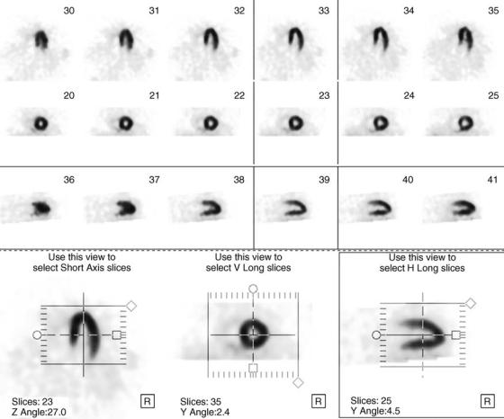
Figure 2. Normal thallium-201 cardiac study. The first three rows show six slices of the left ventricle in three different axes (vertical long axis, short axis, horizontal long axis) of the heart. The fourth row shows how the images can be reoriented along each axis.
Once the final set of pictures are ready for clinical use, then it is the computer that is used for image display and analysis. The computer is also used for storage of the clinical studies and to allow their use by multiple readers at various sites and time points during patient care as required for optimal usage of the diagnostic information they provide. They are also very useful in research aimed at optimizing imaging strategies and systems, and in the education and training of medical personnel.
NM IMAGING
Computers play an essential role in NM as an integral part of the most common imaging device used in NM, which is a gamma camera, and in the obtention of slices through the body made in emission computerized tomography (ECT). Emission CT is the general term referring to the computerbased technique by which the 3D distribution of a radioactive tracer in the human body is obtained and presented as a stack of 2D slices. The acronym ECT should not be confused with CT (for computerized tomography), which refers to imaging using X rays. Historically, the use of two different kinds of radioactive tracers has led to the parallel
evolution of two types of ECT techniques: Single-photon emission computerized tomography (SPECT) and positron emission tomography (PET). The SPECT technology is used with gamma emitters, that is, unstable nuclei whose disintegration led to the emission of high energy photons, called g rays. Gamma rays are just like X rays except that X rays are emitted when electrons loose a good amount of energy and g rays are emitted when energy is given off as a photon or photons during a nuclear disintegration, or when matter and antimatter annihilate. As the name implies, the gamma camera is used with gamma emitters in planar imaging (scintigraphy) where 2D pictures of the distribution of activity within a patients body are made. An illustration of a three-headed SPECT system is shown in Fig. 4. The evolution of SPECT systems has led to a configuration with one, then two and three detectors that are gamma-camera heads. The positron emission tomography is used with emitters whose disintegration results in the emission of a positron (a particle similar to an electron, but with the opposite charge making it the antiparticle to the electron). When a positron that has lost all of its kinetic energy hits an electron, the two annihilate and two photons are emitted from the annihilation. These two photons have the same energy (511 keV) and opposite directions. To

NUCLEAR MEDICINE, COMPUTERS IN |
109 |
detect these two photons, a natural configuration for a PET system is a set of rings of detectors. The two points of detection of the opposite detectors form a line, called the line of response (LOR). A state-of-the-art PET system combined with an X-ray CT system (PET/CT) is shown in Fig. 5.
A gamma camera has three main parts: the scintillating crystal, the collimator, and the photomultiplier tubes (PMT) (Fig. 6). When the crystal (usually thallium-activated sodium iodide) is struck by a high energy photon (g or X ray), it emits light (it scintillates). This light is detected by an array of PMT located at the back of the camera. The sum of the currents emitted by all the PMT after one scintillation is proportional to the energy of the incoming
Figure 3. The FDG study for a patient with lung cancer. Upper to lower rows: transverse, sagittal, and coronal slices.
photon, so the g rays can be sorted according to their energy based upon the electrical signal they generate. Because, for geometrical reasons, the PMT closer to the scintillation see more light than the PMT located farther away, the relative amounts of current of the PMT are used to locate the scintillation. This location alone would be of little use if the direction of the incoming photon was not known. The current way to know the direction is by using a collimator. The collimator is a piece of lead with one or more holes, placed in front of the scintillating crystal, facing the patient. Although different kinds of collimators exist, they are all used to determine, for each incoming photon, its direction before its impact on the crystal. To understand the role of the collimator, one can use the analogy of the gamma-camera with a camera that takes photographs. The
Figure 4. A three-headed SPECT system with the third head below the imaging bed the patient lays on.
Figure 5. Illustration of a state-of-the-art PET/CT system (Philips Medical Systems) with patient bed. The CT system is the first ring-shaped gantry and the PET system is the second ring-shaped gantry. (Reproduced with permission of Philips Medical Systems.)

110 NUCLEAR MEDICINE, COMPUTERS IN
Figure 6. Main parts of a SPECT camera and basic principle. A gamma photon going through the holes of the collimator strikes the crystal. The crystal restitutes the energy of the gamma photon byscintillation, that is, by emitting some transient ultraviolet (UV) light. Some of the UV light is collected by photomultiplier tubes, whose function is to ensure the transduction of the signal (i.e., the conversion of light into electricity). The location of the scintillation and the energy ofthephotonare estimated, digitized and sent to the computer.
collimator plays the role of the objective lens in a camera. An image acquired without a collimator would be totally blurry, as would be a photograph taken with a camera with no lens. This is because g rays are emitted in all directions with equal probabilities, and without a collimator, the photons emitted from a radioactive point source would strike the detector almost uniformly. With a collimator, only the photons whose direction is parallel to the axis of the holes may be potentially detected, while others are stopped by the lead. As a result, the image of a source is (ideally) the projection of the source distribution onto the crystal plane (Fig. 7). Gamma rays can be stopped or scattered, but due to their high penetrating power, it is very difficult to bend them like light rays with lenses, and this is the reason why collimators are used instead of lenses. Photons emitted at different distances from the camera, but along the same direction parallel to a hole, are detected at the same location in the crystal. Thus, the image obtained is the projection of the 3D distribution of the tracer onto the 2D plane of the detector. In that sense, a projection is similar to a chest X ray, in which the images of all the organs (ribs, heart, spine, etc.) are overlaid on the film even though organs do not spatially overlap in the body. The overlay might not be a problem for relatively thin parts of the body, such as a hand, or when tracer-avid structures do not overlap, such as the skeleton. In that case, only one projection is obtained from the best angle of view for the gamma-camera head. As stated above, this technique is called planar imaging, or scintigraphy. However, for other thicker organs like the myocardium and the brain, for which one is interested in measuring the 3D tracer inner distribution, more information is gathered by rotating the heads to acquire projections from multiple angles of view (tomographic acquisition, presented later in this article).
In PET scanners, hundreds of small crystals arranged in rings are used so that the data can be simultaneously acquired along multiple LOR (Fig. 8). Thousands of photons hit the crystals every second, so how to know which two photons are the result of the same electronpositron annihilation? If two photons are detected almost simultaneously, chances are that they are of the same pair (it is called a true coincidence), so an electronic circuitry checks whether one photon is detected 10 ns (the time window) at most after the previous one. It may happen that, although two photons are detected within that time window, they are not of the same pair, and such an event is called a random coincidence. Because in PET the direction of the photons is known (it is the LOR), collimators are not needed; however, because of the limited counting rate capabilities of older systems, septa made of lead may be used to limit the acquisition to the LORs roughly perpendicular to the axial direction, inside the same ring (2D acquisition). With modern PET systems having a high couting rate capability, a 3D acquisition is possible by detecting LORs even when the two photons hit crystals of different rings.
The computer plays an important role in the formation of the image coming from the gamma camera. As described above, the crystal is viewed by an array of 37 to > 100, depending on the model, of PMT. These are analog devices that can drift with time. Also the positioning in the image of the location of the flash of light when a g ray is absorbed in the crystal depends to some extent on where the ray interacts relative to the array of PMT. Such local variations lead to nonuniformity (uneven apparent sensitivity) and
|
Figure 8. Main parts of a PET system. Pairs of photons are |
|
detected in coincidence following the annihilation of a positron |
Figure 7. The role of the collimator in a SPECT system. |
with an electron. |
nonlinearity (straight lines of activity are bent in the image). Prior to the incorporation of computers into the gamma camera electronics, the impact of such local variations was minimized by allowing the light to spread out before reaching the PMT by passing it through a light guide. This resulted in more PMT receiving enough light to participate in determining the location of the interaction thus improving uniformity and linearity, but at the expense of spatial resolution (i. e., determination of where in the crystal the flash of light originated). Modern gamma cameras incorporate computers to correct for local variations in camera performance so that the light guide is virtually eliminated. This in turn has improved spatial resolution.
Computer correction of the camera image usually takes place in three steps (5). The first is energy correction. As we said, the total magnitude of the signal from all the PMT is related to the energy deposited in the crystal by the g ray. However, if a large number of g rays of exactly the same energy interact in the crystal, the magnitude of the electrical signal will vary due to the statistics of turning the light emitted into an electrical signal and local variation in camera performance. By placing a source that will uniformly irradiate the crystal, such as the commercial sheet source shown in Fig. 9, the local variation on average in the magnitude of the signal can be determined on a pixel by pixel basis by computer. The centering of the window employed to select electrical pulses for inclusion in image formation can then be adjusted to give a more uniform response.
Besides varying in the average size of the total electrical pulse detected from the PMT locally, gamma cameras vary in how well they map the true location of the flash of light into its perceived location in the image. Thus, in some regions, detected events are compressed together and in others they are spread apart. Correction of this nonlinear mapping constitutes the second step in computer correction of the gamma-camera image and is called linearity correction. Linearity correction is performed by placing an attenuating sheet with an exactly machined array of very small holes in a precise location between the gamma
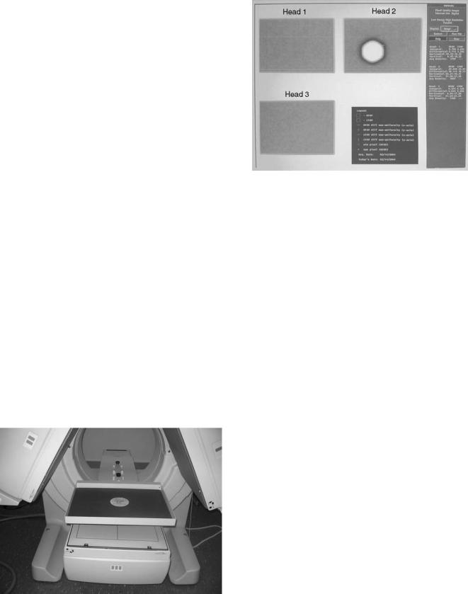
Figure 9. Radioactive sheet source in front of the third head of a three-headed SPECT system in position for checking uniformity and loading correction factors.
NUCLEAR MEDICINE, COMPUTERS IN |
111 |
Figure 10. Output from checking camera uniformity when a single PM on head 2 of the three-headed SPECT system of Fig. 9 has failed.
camera and the sheet source of Fig. 9. A high resolution image consisting of a large number of gamma-ray events is then acquired. The images of the holes do not match where they should appear. The vector displacement of the image of the hole back to its true location defines how the mapping from true to detected location is inaccurate at that location. By using the computer to interpolate between the array of measured distortions at the pixel level, a map is generated giving how each event detected at a location in the crystal should be displaced in the resulting image.
The final step in image correction is called flood correction. If an image of a large number of events from a sheet source is acquired with energy and linearity correction enabled, then any residual nonuniformity is corrected by determining with computer a matrix that when multiplied by this image would result in a perfectly uniform image of the same number of counts. This matrix is then saved and used to correct all images acquired by the gamma camera before they are written to disk.
An example of testing camera uniformity is shown in Fig. 10. Here again, a sheet source of radioactivity is placed in front of the camera head as shown in Fig. 9. High count images of the sheet source are inspected numerically by computer and visually by the operator each day before the camera is employed clinically. Heads 1 and 3 in Fig. 10 show both numerically and visually good uniformity. A large defect is seen just below and to the left of center in the image from head 2. This is the result of the failure of a single PMT. A single PMT affects a region much larger than its size because it is the combined output of all the PMT close to the interation location of a gamma-ray that are used to determine its location.
Images can be classified in two types, mutually exclusive: analog or digital. A chest X ray on a film is a typical example of an analog image. Analog images are not divided into a finite number of elements, and the values in the image can vary continuously. An example of digital image is a photograph obtained with a digital camera. Much like roadmaps, a digital image is divided into rows and columns, so that it is possible to find a location given its row
112 NUCLEAR MEDICINE, COMPUTERS IN
Figure 11. Left: example of an 8 8 image. Each square represents a pixel. The dark gray borders of each square have been added here for sake of clarity, but are not present in the image when stored on the computer. Each pixel has a level of gray attached to it. Right: the values in each pixel. In its simplest form, the image is stored in a computer as a series of lexicographically ordered values. The rank of each value in the series defines the pixel location in the image (e.g., the 10th value of the series refers to the 10th pixel of the image). There is a 1:1 relationship between the brightness and the value. The correspondence between the color and the value is defined in a table called look-up table (LUT) or a color map. An image can be a shade of grays (black and white) or in color.
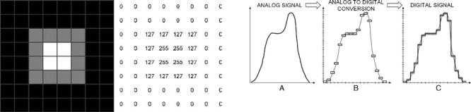
and column. The intersection of a row and a column defines one picture element, or pixel, of the image. Each pixel has a value that usually defines its brightness, or its color. A digital image can be seen as a rectangular array of values (Fig. 11), and thus be considered, from a mathematical point of view, as a matrix. Computers cannot deal with analog values, so whenever an analog measurement (here, the current pulse generated after the impact of a gamma photon in the crystal) is made, among the first steps is the analog-to-digital conversion (ADC), also called digitization. The ADC is the process during that an infinite number of possible values is reduced to a limited (discrete) number of values, by defining a range (i.e., minimum and maximum values), and dividing the range into intervals, or bins (Fig. 12). The performance of an ADC is defined by its ability to yield a digital signal as close as possible to the analog input. It is clear from Fig. 12 that the digitized data are closer to the analog signal when the cells are smaller. The width of the cells is defined by the sampling rate, that is, the number of measurements the ADC can convert per unit of time. The height of the cells is defined by the resolution of the ADC. A 12-bit resolution means that the ADC sorts the amplitude of the analog values among one of 212 ¼ 4096 possible values. The ADC has also a range, that is, the minimum and maximum analog amplitudes it can handle. For example, using a 12-bit analog-to- digital converter with a 10 to þ10 V range (i.e., a 20 V range), the height of each cell is 20/4096 (i.e., 0.005 V). Even if the analog signal is recorded with a 0.001 V accuracy, after ADC the digital signal accuracy will be at best 0.005 V. The point here is that any ADC is characterized by its sampling rate, its resolution and its range. Both the SPECT and PET systems measure the location and the energy of the photons hitting their detectors. The measurements are initially analog, and are digitized as described above before being stored on a computer. In SPECT, prior
Figure 12. (a) Example of an analog signal, for example the intensity of gray (vertical axis) along a line (horizontal axis) drawn on a photograph taken with a nondigital camera. (b) The process of ADC, for example when the photograph is scanned to be archived as an image file on a computer. The 2D space is divided into a limited number of rectangular cells as indicated by the tick marks on both axes. For sake of clarity, only the cells whose center is close to the analog signal are drawn in this figure, and this set of cells is the result of the ADC. (c) The digital signal is drawn by joining the center of the cells, so that one can compare the two signals.
to the beginning of the acquisition, the operator chooses the width and height (in pixels) of the digital image to be acquired. Common sizes are 64 by 64 pixels (noted 64 64, width by height), 128 128 or 256 256. Dividing the size of the field of view (in cm) by the number of pixels yields the pixel size (in cm). For example, if the usable size for the detector is 40 40 cm, the pixel size is 40/64 ¼ 0.66 cm for a 64 64 image. Because all devices are imperfect, a point source is seen as a blurry spot on the image. If two radioactive point sources in the field of view are close enough, their spots overlap each other. When the two sources get closer, at some point the spots cannot be visually separated in the image. The smallest distance between the sources that allows us to see one spot for each source is called the spatial resolution. The pixel size is not to be confused with the spatial resolution. While the pixel size is chosen by the operator, the spatial resolution is imposed by the camera characteristics, and most notably by the collimator now that thick light guides are no longer employed. The pixel size is chosen to be smaller than the resolution, so that we can get as much detail as the resolution allows us to get, but it is important to understand that using a pixel size much smaller than the resolution does not increase the image quality. If the pixel size is small (i.e., when the number of pixels in the field of view is large), then the spot spills over many pixels, but with no improvement to image resolution.
The energy resolution (i.e., the smallest change in energy the detector can measure) is limited, and its value has a great impact on image quality, as explained below. Between the points of emission and detection, photons with an energy < 1 MeV frequently interact with electrons by scattering, during which their direction changes and some of their energy is lost. Because their direction changes, an error is made on their origin. However, it is possible to know that a photon is scattered because it has lost some energy, so an energy window, called the photopeak window defined around the energy of nonscattered (primary) photons (the photopeak), is defined prior to the acquisition, and the scattered photons whose energy falls outside the
photopeak window can be identified by energy discrimination and ignored. Unfortunately, photons in the photopeak window can either be scattered photons, or a primary photon whose energy has been underestimated (due to the limited energy resolution of the detectors, an error can be made regarding the actual energy of the photons). If the photopeak window is wide, many scattered photons are accepted, and the image has a lot of scattered activity that reduces the contrast; if the energy window is narrow, many primary photons are rejected, and the image quality is poor because of a lack of signal. As the energy resolution increases, the energy window can be narrowed, so that most scattered photons can be rejected while most primary photons are kept.
As mentioned above, the 3D distribution of the tracer in the field of view is projected onto the 2D plane of the camera heads. As opposed to the list-mode format (presented later in this article), the projection format refers to the process of keeping track of the total number of photons detected (the events, or counts) for each pixel of the projection image. Each time a count is detected for a given pixel, a value of 1 is added to the current number of counts for that pixel. In that sense, a projection represents the accumulation of the counts on the detector for a given period of time. If no event is recorded for any given pixel, which is not uncommon especially in the most peripheral parts of the image, then the value for that pixel is 0. Usually, 16 bits (2 bytes) are allocated to represent the number of counts per pixel, so the range for the number of events is 0 to 216 1 ¼ 65,535 counts per pixel. In case the maximal value is reached for a pixel (e.g., for a highly active source and a long acquisition time), then the computer possibly stops incrementing the counter, or reinitializes the pixel value to 0 and restarts counting from that point on. This yields images in which the most radioactive areas in the image may paradoxically have a lower number of counts than surrounding, less active, areas.
Different acquisitions are possible with a gamma camera: Planar (or static): The gamma-camera head is stationary. One projection is obtained by recording the location of the events during a given period from a single angle of view. This is equivalent to taking a photograph with a camera. The image is usually acquired when the tracer uptake in the organ of interest has reached a stable level. One is interested in finding the quantity of radiopharmaceutical that accumulated in the region of interest. Planar images are usually adequate for thin or small structures (relative to the resolution of the images), such
as the bones, the kidneys, or the thyroid.
Whole body: This acquisition is similar to the planar acquisition, in the sense that one projection is obtained per detector head, but is designed, as the name implies, to obtain an image of the whole body. Since the human body is taller than the size of the detector ( 40 40 cm), the detector slowly moves from head to toes. This exam is especially indicated when looking for metastases. When a cancer starts developing at a primary location, it may happen that
NUCLEAR MEDICINE, COMPUTERS IN |
113 |
cancer cells, called metastases, disseminate in the whole body, and end up in various locations, especially bones. There, they may start proliferating and a new cancer may be initiated at that location. A whole-body scintigraphy is extremely useful when the physician wants to know whether one or more secondary tumors start developing, without knowing exactly where to look at.
Dynamic: Many projections are successively taken, and each of them is typically acquired over a short period (a few seconds). This is equivalent to recording of a movie. Analyzing the variations as a function of time allows us to compute parameters, such as the uptake rate, which can be a useful clinical index of normality.
Gated: The typical application of a gated acquisition is the cardiac scintigraphy. Electrodes are placed on the patient’s chest to record the electrocardiogram (ECG or EKG). The acquisition starts at the beginning of the cardiac cycle, and a dynamic sequence of 8 or 16 images is acquired over the cardiac cycle ( 1 s), so that a movie of the beating heart is obtained. However, the image quality is very poor when the acquisition is so brief. So, the acquisition process is repeated many times (i.e., over many heart beats), and the first image of all cardiac cycles are summed together, the second image of all cardiac cycles are summed together, and so on.
Tomographic: The detector heads are rotating around the patient. Projections are obtained under multiple angles of view. Through a process called tomographic reconstruction (presented in the next section), the set of 2D projections is used to find the 3D distribution of the tracer in the body, as a stack of 2D slices. The set of 1D projections of one slice for all projection angles is called a sinogram.
Tomographic gated: As the name implies, this acquisition is a tomographic one with gating information. The ECG is recorded during the tomographic acquisition, and for each angle of view, projections are acquired over many cardiac cycles, just as with a gated acquisition (see above). Thus, a set of projections is obtained for each point of the cardiac cycle. Each set is reconstructed, and tomographic images are obtained for each point of the cardiac cycle.
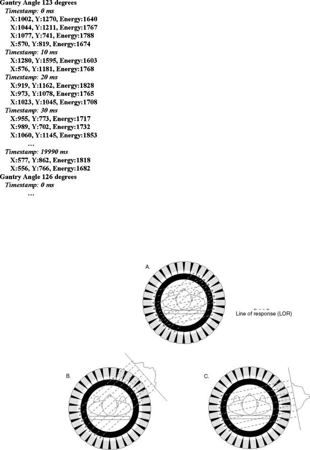
In contrast with the types of acquisition above in which the data are accumulated in the projection matrix for several seconds or minutes (frame-mode acquisition), a much less frequent type of acquisition called list-mode acquisition, can also be useful, because more information is available in this mode. As the name implies, the information for each individual event is listed in the list-mode file, and are not arranged in a matrix array. In addition to the coordinates of the scintillations, additional data are stored in the file. Figure 13 illustrates the typical listmode format for a SPECT system. List-mode information is similar with a PET system, except that the heads location and X–Y coordinates are replaced with the location of the event on the detector rings. The list-mode file ( 50 Mb
114 NUCLEAR MEDICINE, COMPUTERS IN
Figure 13. Example of data stored on-the-fly in a list-mode file data in a SPECT system. Gantry angle defines the location of the detectors. The X and Y coordinates are given in a 2048 2048 matrix. The energy is a 12-bit value (i.e., between 0 and 4,095), and a calibration is required to convert these values in usual units (i.e., kiloelectron volt, keV).
in size in SPECT) can be quite large relative to a projection file. The list-mode format is far less common than the projection format, because it contains information, such as timing, that would usually not be used for a routine clinical exam. The list-mode data can be transformed into projection data through a process called rebinning (Fig. 14). Since the timing is known, multiple projections can be created as a function of time, thus allowing the creation of ‘‘movies’’ whose rate can be defined postacquisition. A renewed interest in the list-mode format has been fueled these past years by the temporal information it contains, which is adequate for the temporal correlation of the acquisition with patient, cardiac, or respiratory motions through the synchronized acquisition of signal from motion detectors.
TOMOGRAPHIC RECONSTRUCTION
Tomographic reconstruction has played a central role in NM, and has heavily relied on computers (6). In addition to data acquisition control, tomographic reconstruction is the other main reason for which computers have been early introduced in NM. Among all uses of computers in NM, tomographic reconstruction is probably the one that symbolizes most the crunching power of computers. Tomographic reconstruction is the process by which slices of the 3D distribution of tracers are obtained based upon the projections obtained under different angles of view. Because the radioactivity emitted in the 3D space is projected on the 2D detectors, the contrast is usually low. Tomographic reconstruction greatly restores the contrast, by estimating the 3D tracer distribution. Reconstruction is possible using list-mode data (SPECT or PET), but mainly
Figure 14. Rebinning process. (a) The line joining pairs of photons detected in coincidence is called a line of response (LOR). (b and c) LOR are sorted so that parallel LOR are grouped, for a given angle.
NUCLEAR MEDICINE, COMPUTERS IN |
115 |
for research purposes. The PET data, although initially acquired in list-mode format, are usually reformatted to form projections, so that the algorithms developped in SPECT can also be used with PET data. There are many different algorithms, mainly the filtered back-projection (FBP) and the iterative algorithms, that shall be summarized below (7–9).
In the following, focuses on tomographic reconstruction when input data are projections, which is almost always the caseon SPECTsystems.During aSPECTacquisition, the detecting heads rotate around the subject to gather projections from different angles of views (Fig. 15). Figure 16 presents the model used to express the simplified projection process in mathematical terms. Associated with the projection is the backprojection (Fig. 17). With backprojection, the activity in each detector bin g is added to all the voxels which project onto bin g. It can be shown (10) that backprojecting projections filtered with a special filter called a ramp filter (filtered backprojection, or FBP) is a way to reconstruct slices. However, the ramp filter is known to increase the high frequency noise, so it is usually combined with a low pass filter (e.g., Butterworth filter) to form a band-pass filter. Alternatively, reconstruction can be performed with the ramp filter only, and then the reconstructed images can be smoothed with a 3D low pass filter. The FBP technique yields surprisingly good results considering the simplicity of the method and its approximations, and is still widely used today. However, this rather crude approach is more and more frequently replaced by the more sophisticated iterative algorithms, in which many corrections can be easily introduced to yield
Figure 15. The SPECT acquisition. Left. A threehead IRIX SPECT system (Philips Medical Systems). A subject is in the field of view while the camera heads are slowly rotating around him. Right. Physical model and geometric considerations. The 2D distribution of the radioactivity f(x,y) in one slice of the body is projected and accumulated onto the corresponding 1D line g(s,u) of detector bins.
more accurate results. An example of an iterative reconstruction algorithm includes the following steps:
1.An initial estimate of the reconstructed is created, by attributing to all voxels the same arbitrary value (e.g. 0 or 1).
2.The projections of this initial estimate are computed.
3.The estimated projections are compared to the measured projections, either by computing their difference or their ratio.
4.The difference (resp. the ratio) is added (resp. multiplied) to the initial estimate to get a new estimate.
5.Steps 2–4 are repeated until the projections of the current estimate are close to the measured projections.
Figure 18 illustrates a simplified version of the multiplicative version of the algorithm. This example has been voluntarily oversimplified for sake of clarity. Indeed, image reconstruction in the real world is much more complex for several reasons: (1) images are much larger; typically, the 3D volume is made of 128 128 128 voxels, (2) geometric considerations are included to take into account the volume of each volume element (voxel) that effectively project onto each bin at each angle of view, (3) camera characteristics, and in particular the spatial resolution, mainly defined by the collimator characteristics, are introduced in the algorithm, and (4) corrections presented below are applied during the iterative process. The huge number of operations made iterative reconstruction a slow process and prevented its routine use until recently, and FBP was
Figure 16. Projection. Each plane in the FOV (left) is seen as a set of values f (center). The collimator is the device that defines the geometry of the projection. The values in the projections are the sum of the values in the slices. An example is presented (right). (Reproduced from Ref. 8 with modifications with permission of the Society of Nuclear Medicine Inc.)

116 NUCLEAR MEDICINE, COMPUTERS IN
Figure 17. Projection and backprojection. Notice that backprojection is not the invert of projection. (Reproduced from Ref. 8 with modifications with permission of the Society of Nuclear Medicine Inc.)
preferred. Modern computers are now fast enough for iterative algorithms, and since these algorithms have many advantages over the FBP, they are more and more widely used.
A number of corrections usually need to be applied to the data during the iterative reconstruction to correct them for various well-known errors caused by processes associated with the physics of the detection, among which the more important are attenuation (11–13), Compton scattering (11,12), depth-dependent resolution (in SPECT) (11,12), random coincidences (in PET) (14), and partial volume effect (15). These sources of error below are briefly presented:
Attenuation occurs when photons are stopped (mostly in the body), and increases with the thickness and the density of the medium. Thus, the inner parts of the body usually appear less active than the more superficial parts (except the lungs, whose low density makes them almost transparent to gamma photons and appear more active than the surrounding soft tissues). Attenuation can be compensated by multiplying the activity in each voxel by a factor whose value depends upon the length and the density of the tissues encountered along the photons path. The correction factor can be estimated (e.g., by assuming a uniform attenuation map) or measured using an external radioactive source irradiating the subject. A third possibility, which is especially attractive with the advent of SPECT/CT and PET/CT systems (presented below), is to use the CT images to estimate the attenuation maps.
Photons may be scattered when passing through soft tissues and bones, and scattered photons are deflected from their original path. Because of the error in the estimated origin of the scattered photons, images are slightly blurred and contrast decreases. As mentioned in the previous section, the effects of scattering can be better limited by
Figure 18. A simplified illustration of tomographic reconstruction with an iterative algorithm. (a) The goal is to find the values in a slice (question marks) given the measured projection values 7, 10, 3, 6, 9, 5. (b) Voxels in the initial estimate have a value of 1, and projections are computed as described in Fig. 17. (c) The error in the projections is estimated by dividing the actual values by the estimated values. The ratios are then backprojected to get a slice of the ‘‘error’’. (d) Multiplying the error obtained in c by the estimate in b yields a second estimate, and projections are computed again
(g). After an arbitrary number of iterations (e, f), an image whose projections are close to the measured projections is obtained. This image is the result of the iterative tomographic reconstruction process. Such a process is repeated for the stack of 2D slices.
using detectors with a high energy resolution. Scatter can also be estimated by acquiring projection data in several energy windows during the same acquisition. Prior to the acquisition, the user defines usually two or three windows per photopeak (the photopeak window plus two adjacent windows, called the scatter windows). As mentioned, photons can be sorted based upon their energy, so they can be assigned to one of the windows. The amount of scattering is estimated in the photopeak window using projection data acquired in the scatter windows, and assuming a known relationship between the amount of scattering and the energy. Another approach to Compton scattering compensation uses the reconstructed radioactive distribution and attenuation maps to determine the amount of scatter using the principles of scattering interactions.
In SPECT, collimators introduce a blur (i.e., even an infinitely small radioactive source would be seen as a spot of several mm in diameter) for geometrical reasons. In addition, for parallel collimators (the most commonly used, in which the holes are parallel), the blur increases as the distance between the source and the collimator increases. Depth-dependent resolution can be corrected either by fil-
tering the sinogram in the Fourier domain using a filter whose characteristics vary as a function of the distance to the collimator (frequency–distance relationship, FDR) or by modelling the blur in iterative reconstruction algorithms.
In PET, a coincidence is defined as the detection of two photons (by different detectors) in a narrow temporal window of 10 ns. As mentioned, a coincidence is true when the two photons are of the same pair, and random when the photons are from two different annihilations. The amount of random coincidences can be estimated by defining a delayed time window, such that no true coincidence can be detected. The estimation of the random coincidences can then be subtracted from the data including both true and random, to extract the true coincidences.
Partial volume effect (PVE) is directly related to the finite spatial resolution of the images: structures that are small (about the voxel size and smaller) see their concentration underestimated (the tracer in the structure appears as being diluted in the voxel). Spillover is observed at the edges of active structures: some activity spreads outside the voxels, so that although it stems from the structure, it is actually detected in neighboring voxels. Although several techniques exist, the most accurate can be implemented when the anatomical boundaries of the structures are known. Thus, as presented below, anatomical images from CT scanners are especially useful for PVE and spillover corrections, if they can be correctly registered with the SPECT or PET data.
IMAGE PROCESSING, ANALYSIS AND DISPLAY
Computers are essential in NM not only for their ability to control the gamma cameras and to acquire images, but also because of their extreme ability to process, analyze and display the data. Computers are essential in this respect because (1) the amount of data can be large (millions of pixel values), and computers are extremely well suited to handle images in their multimegabytes memory, (2) repetitive tasks are often needed and central processor units (CPUs) and array processors can repeat tasks quickly, (3) efficient algorithms have been implemented as computer programs to carry on complex mathematical processing, and (4) computer monitors are extremely convenient to display images in a flexible way.
Both the PET and SPECT computers come with a dedicated, user-friendly graphical environment, for acquisition control, patient database management, and a set of programs for tomographic reconstruction, filtering and image manipulation. These programs are usually written in the C language or in Fortran, and compiled (i.e., translated in a binary form a CPU can understand) for a given processor and a given operating system (OS), usually the Unix OS (The Open Group, San Francisco CA) or the Windows OS (Microsoft Corporation, Redmond WA). As an alternative to these machine-dependent programs, Java (Sun Microsystems Inc.) based programs have been proposed (see next section).
As seen in the first section, an image can be seen as a rectangular array of values, which is called, from a mathematical point of view, a matrix. A large part of image
NUCLEAR MEDICINE, COMPUTERS IN |
117 |
processing in NM is thus based upon linear algebra (16), which is the branch of mathematics that deals with matrices. One of the problems encountered in NM imaging is the noise (random variations due to the probabilistic nature of the radioactive processes and to the limited accuracy of the measurements). A number of methods are available to reduce the noise after the acquisition, by smoothing the minor irregularities or speckles in the images (10). The most common way to filter images is by convolution (a pixel value is replaced by a weighted average of its neighbors) or by Fourier methods. Computers are extremely efficient at computing discrete Fourier transforms thanks to a famous algorithm called the fast Fourier transform (FFT) developed by Cooley and Tukey (17).
The NM images can be displayed or printed in black and white (gray levels) or in color. Pixel values can be visually estimated based on the level of gray or based on the color. Color has no special meaning in NM images, and there is no consensus about the best color map to use. Most often, a pixel value represents a number of counts, or events. However, units can be something else (e.g., flow units), especially after some image processing. So, for proper interpretation, color map and units should always accompany an image.
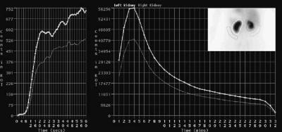
Regions of interest (ROIs) are defined by line segments drawn to set limits in images and can have any shape or be drawn by hand. The computer is then able to determine which pixels of the image are out and which are in the ROI, and thus computations can be restricted to the inside or to the outside of the ROI. ROIs are usually drawn with the mouse, based on the visual inspection of the image. Drawing a ROI is often a tricky task, due to the low resolution of the images and to the lack of anatomical information regarding the edges of the organs. In an attempt to speed up the process, and to reduce the variability among users, ROIs can also be drawn automatically (18). When a dynamic acquisition is available, a ROI can be drawn on one image and reported on the other images of the series, the counts in the ROI are summed and displayed as a time– activity curve (TAC), so that one gets an idea of the kinetics of the tracer in the ROI. The TAC are useful because with the appropriate model, physiological parameters such as pharmacological constants or blood flow can be determined based on the shape of the curve. An example of dynamic studies with ROI and TAC is the renal scintigraphy, whose goal is to investigate the renal function through the vascularization of the kidneys, their ability to filter the blood, and the excretion in the urine. A tracer is administered with the patient lying on the bed of the camera, and a twostage dynamic acquisition is initiated: many brief images are acquired (e.g., 1 image per second over the first 60 s). Then, the dynamic images are acquired at a lower rate (e.g., 1 image per minute for 30 min). After the acquisition, ROIs are drawn over the aorta, the cortical part of the kidneys, and the background (around the kidneys), and the corresponding TAC are generated for analysis (Fig. 19). The TAC obtained during the first stage of the acquisition reflect the arrival of the tracer in the renal arteries (vascular phase). The rate at which the tracer invades the renal vascularization, relative to the speed at which it arrives in the aorta above indicates whether the kidneys
118 NUCLEAR MEDICINE, COMPUTERS IN
Figure 19. Output of a typical renal scintigraphy. Left: the TAC for both kidneys in the first minute after injection of the tracer. The slope of the TAC gives an indication of the state of the renal vascularization. Center: One-minute images acquired over 32 min after injection. The ascending part evidences the active tracer uptake by the kidneys, while the descending part shows the excretion rate. Right: Insert shows the accumulation of the tracer in the bean-shaped kidneys. The ROI are drawn over the kidneys and the background.
are normally vascularized. The renal TAC obtained in the second stage of the acquisition (filtration phase) show the amount of tracer captured by the kidneys, so that the role of the kidneys as filters can be assessed. When the tracer is no longer delivered to the kidneys, and as it passes down the ureters (excretion phase), the latest part of the renal curves normally displays a declining phase, and the excretion rate can be estimated by computing the time of half-excretion (i.e., the time it takes for the activity to decreases from its peak to half the peak), usually assuming the decrease is an exponential function of time.
The corrections presented at the end of the previous section are required to obtain tomographic images in which pixel values (in counts per pixel) are proportional to the tracer concentration with the same proportion factor (relative quantitation), so that different areas in the same volume can be compared. When the calibration of the SPECT or PET system is available (e.g., after using a phantom whose radioactive concentration is known), the images can be expressed in terms of activity per volume unit, (e.g., in becquerels per milliliters, Bq mL 1; absolute quantitation). Absolute quantitation is required in the estimation of a widely used parameter, the standardized uptake value (SUV) (19), which is an index of the FDG uptake that takes into account the amount of injected activity and the dilution of the tracer in the body. The SUV in the region of interest is computed as SUV ¼ (uptake in the ROI in Bq mL 1)/(injected activity in Bq/body volume in mL). Another example of quantitation is the determination of the blood flow (in mL g 1 min 1), based upon the pixel values and an appropriate model for the tracer kinetics in the area of interest. For example, the absolute regional cerebral blood flow (rCBF) is of interest in a number of neurological pathologies (e.g., ischemia, haemorrage, degenerative diseases, epilepsy). It can be determined with xenon 133Xe, a gas that has the interesting property of being washed out from the brain after its inhalation as a simple exponential function of the rCBF. Thus, the rCBF can be assessed after at least two fast tomographic acquisitions (evidencing the differential decrease in activity in the various parts of the brain), for example, using the Tomomatic 64 SPECT system (Medimatic, Copenhagen, Denmark) (20).
An example of image processing in NM is the equilibrium radionuclide angiography (ERNA) (21), also called multiple gated acquisition (MUGA) scan, for assessment of
the left ventricle ejection fraction (LVEF) of the heart. After a blood sample is taken, the erythrocytes are labelled with 99 mTc and injected to the patient. Because the technetium is retained in the erythrocytes, the blood pool can be visualized in the images. After a planar cardiac gated acquisition, 8 or 16 images of the blood in the cardiac cavities (especially in the left ventricle) are obtained during an average cardiac cycle. A ROI is drawn, manually or automatically, over the left ventricle, in the end-diastolic (ED) and end-systolic (ES) frames, that is, at maximum contraction and at maximum dilatation of the left ventricle respectively. Another ROI is also drawn outside the heart for background activity subtraction. The number of counts nED and nES in ED and ES images, respectively, allows the calculation of the LVEF as LVEF ¼ (nED-nES)/nED. Acquisitions for the LVEF assessment can also be tomographic in order to improve the delineation of the ROI over the left ventricle, and several commercial softwares are available (22) for largely automated processing, among which the most widely used are the Quantitative Gated SPECT (QGS) from the Cedars-Sinai Medical Center, Los Angeles, and the Emory Cardiac Tool box (ECTb) from the Emory University Hospital, Atlanta.
INFORMATION TECHNOLOGY
An image file typically contains, in addition to the image data, information to identify the images (patient name, hospital patient identification, exam date, exam type, etc.), and to know how to read the image data (e.g., the number of bytes used to store one pixel value). File format refers to the way information is stored in computer files. A file format can be seen as a template that tell the computer how and where in the file data are stored. Originally, each gammacamera manufacturer had its own file format, called proprietary format, and for some manufacturers the proprietary format was confidential and not meant to be widely disclosed. To facilitate the exchange of images between different computers, the Interfile format (23) was proposed in the late 1980s. Specifically designed for NM images, it was intended to be a common file format that anyone could understand and use to share files. At the same period, the American College of Radiology (ACR) and the National Electrical Manufacturers Association (NEMA) developed their standard for NM, radiology, MRI and ultrasound images: the ACR-NEMA file format, version 1.0 (in 1985)
and 2.0 (in 1988). In the early 1990s, local area networks (LANs) connecting NM, radiology and MRI departments started to be installed. Because Interfile was not designed to deal with modalities other than NM, and because ACRNEMA 2.0 was ‘‘only’’ a file format, and was not able to handle robust network communications to exchange images over a LAN, both became obsolete and a new standard was developed by the ACR and the NEMA, ACR-NEMA 3.0, known as Digital Imaging and Communications in Medicine (DICOM) (24). Although quite complex (the documentation requires literally thousands of pages), DICOM is powerful, general in its scope and designed to be used by virtually any profession using digital medical images. Freely available on the Internet, DICOM has become a standard among the manufacturers, and it is to be noted that DICOM is more than a file format. It also includes methods (programs) for storing and exchanging image information; in particular, DICOM servers are programs designed to process requests for handling DICOM images over a LAN.
DICOM is now an essential part of what is known as Picture Archiving and Communications Systems (PACS). Many modern hospitals use a PACS to manage the images and to integrate them into the hospital information system (HIS). The role of the PACS is to identify, store, protect (from unauthorized access) and retrieve digital images and ancillary information. A web server can be used as an interface between the client and the PACS (25). Access to the images does not necessarily require a dedicated software on the client. A simple connection to the Internet and a web browser can be sufficient, so that the images can be seen from the interpreting or prescribing physician’s office. In that case, the web server is responsible for submitting the user’s request to the PACS, and for sending the image data provided by the PACS to the client, if the proper authorization is granted. However, in practice, the integration of NM in a DICOM-based PACS is difficult, mainly because PACS evolved for CT and MR images (26,27), that is, as mostly static, 2D, black and white images. The NM is much richer from this point of view, with different kinds of format (list-mode, projections, whole-body, dynamic, gated, tomographic, tomographic gated, etc.) and specific postacquisition processing techniques and dynamic displays. The information regarding the colormaps can also be a problem for a PACS when dealing with PET or SPECT images fused with CT images (see next section) because two different colormaps are used (one color, one grayscale) with different degrees of image blending.
In the spirit of the free availability of programs symbolized by the Linux operating system, programs have been developed for NM image processing and reconstruction as plug-ins to the freely available ImageJ program developed at the U.S. National Institutes of Health (28). ImageJ is a general purpose program, written with Java, for image display and processing. Dedicated Java modules (plugs-in) can be developed by anyone and added as needed to perform specific tasks, and a number of them are available for ImageJ (29). Java is a platform-independent language, so that the same version of a Java program can run on different computers, provided that another program, the Java virtual machine (JVM), which is platform-dependent,
NUCLEAR MEDICINE, COMPUTERS IN |
119 |
has been installed beforehand. In the real world, however, different versions of the JVM may cause the Java programs to crash or to cause instabilities when the programs require capabilities the JVM cannot provide (30). The advantage of the Java programs is that they can be used inside most Internet browsers, so that the user has no program to install (except the JVM). A Java-based program called JaRVis (standing for Java-based remote viewing station) has been proposed in that spirit for viewing and reporting of nuclear medicine images (31).
It is very interesting to observe how, as the time goes by, higher levels of integration have been reached: with the early scintigraphy systems, such as rectilinear scanners (in the 1970s), images were analog, and the outputs were film or paper hard copies. In the 1980s images were largely digital, but computers were mainly stand alone machines. One decade later, computers were commonly interconnected through LANs, and standard formats were available, permitting digital image exchange and image fusion (see next section). Since the mid-1990s, PACS and the worldwide web make images remotely available, thus allowing telemedecine.
HYBRID SPECT/CT AND PET/CT SYSTEMS
Multimodality imaging (SPECT/CT and PET/CT) combines the excellent anatomical resolution of CT with SPECT or PET functional information (2,3). Other advantages of multimodality are (1) the use of CT images to estimate attenuation and to correct for PVE in emission images, (2) the potential improvement of emission data reconstruction by inserting in the iterative reconstruction program prior information regarding the locations of organ and/or tumor boundaries, and (3) the possible comparison of both sets of images for diagnostic purposes, if the CT images are of diagnostic quality. The idea of combining information provided by two imaging modalities is not new, and a lot of work has been devoted to multimodality. Multimodality initially required that the data acquired from the same patient, but on different systems and on different occasions, be grouped on the same computer, usually using tapes to physically transfer the data. This was, 20 years ago, a slow and tedious process. The development of hospital computer network in the 1990s greatly facilitated the transfer of data, and the problem of proprietary image formats to be decoded was eased when a common format (DICOM) began to spread. However, since the exams were still carried out in different times and locations, the data needed to be registered. Registration can be difficult, especially because emission data sometimes contain very little or no anatomical landmarks, and external fiducial markers were often needed. Given the huge potential of dualmodality systems, especially in oncology, a great amount of energy has been devoted in the past few years to make it available in clinical routine. Today, several manufacturers propose combined PET/CT and SPECT/CT hybrid systems (Fig. 20): The scanners are in the same room, and the table on which the patient lies can slide from one scanner to the other (Fig. 21). An illustration of PET/CT images is presented in Fig. 22.
120 NUCLEAR MEDICINE, COMPUTERS IN
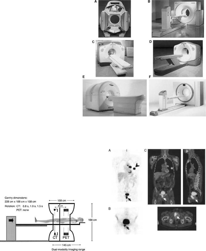
Figure 20. Current commercial PET/CT scanners from 4 major vendors of PET imaging equipment: (a) Hawkeye (GE Medical Systems); (b) Biograph (Siemens Medical Solutions) or Reveal (CTI, Inc);
(c) Discovery LS (GE Medical Systems); (d) Discovery ST (GE Medical Systems); (e) Gemini (Philips Medical Systems); (f) Biograph Sensation 16 (Siemens Medical Solutions) or Reveal XVI (CTI, Inc.). (Reproduced from Ref. 2, with permission of the Society of Nuclear Medicine Inc.)
Although patient motion is minimized with hybrid systems, images from both modalities are acquired sequentially, and the patient may move between the acquisitions, so that some sort of registration may be required before PET images can be overlaid over CT images. Again, computer programs play an essential role in finding the best correction to apply to one dataset so that it matches the other dataset. Registration may be not too difficult with relatively rigid structures, such as the brain, but tricky for chest imaging for which nonrigid transformations are needed. Also, respiratory motion introduces in CT images mushroom-like artifacts that can be limited by asking the patients to hold their breath at midrespiratory cycle during CT acquisition, so that it best matches the average images obtained in emission tomography with no respiratory gating.
Dedicated programs are required for multimodality image display (1) to match the images (resolution, size, orientation); (2) to display superimposed images from both modalities with different color maps (CT data are
Figure 21. Schematic of PET/CT developped by CPS Innovations. Axial separation of two imaging fields is 80 cm. The coscan range for acquiring both PET and CT has maximum of 145 cm. (Reproduced from Ref. 2, with permission of the Society of Nuclear Medicine Inc.)
Figure 22. Image of a 66 years old male patient with history of head-and-neck cancer. In addition to 18FDG uptake in lung malignancy, intense uptake is seen on PET scan (a) in midline, anterior and inferior to bladder. Note also presence of lung lesion (arrowhead) due to primary lung cancer. 99mTc bone scan (b) subsequently confirmed that uptake was due to metastatic bone disease. PET/CT scan (c) directly localized uptake to pubic ramus (arrowed). (Reproduced from Ref. 2, with permission of the Society of Nuclear Medicine Inc.)
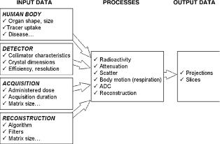
typically displayed with a gray scale, while a color map is used to display the tracer uptake); (3) to adjust the degree of transparency of each modality relative to the other in the overlaid images; and (4) to select the intensity scale that defines the visibility of the bones, soft tissues and lungs in the CT images. For the interpretation of SPECT/CT or PET/CT data, the visualization program has to be optimized, for so much information is available (dozens of slices for each modality, plus the overlaid images, each of them in three perpendicular planes) and several settings (slice selection, shades of gray, color map, the degree of blending of the two modalities in the superimposed images) are to be set. Powerful computers are required to be able to handle all the data in the computer random access memory (RAM) and to display them in real time, especially when the CT images are used at their full quality (512 512 pixel per slice, 16-bit shades of gray). Finally, these new systems significantly increase the amount of data to be archived (one hundred to several hundreds megabytes per study), and some trade-off may have to be found between storing all the information available for later use and minimizing the storage space required. An excellent review of the current software techniques for merging anatomic and functional information is available (32).
COMPUTER SIMULATION
Simulation is a very important application of computers in NM research, as it is in many technical fields today. The advantage of simulation is that a radioactive source and a SPECT or PET system are not required to get images similar to the ones obtained if there were real sources and systems. Simulation is cheaper, faster and more efficient to evaluate acquisition hardware or software before they are manufactured and to change its design for optimization. Thus, one of the applications is the prediction of the performance of a SPECT or PET system by computer simulation. Another application is to test programs on simulated images that have been created in perfectly known conditions, so that the ouput of the programs can be predicted and compared to the actual results to search for possible errors.
Computer simulation is the art of creating information about data or processes without real measurement devices, and the basic idea is the following: if enough information is provided to the computer regarding the object of study (e.g., the 3D distribution of radioactivity in the body, the attenuation), the imaging system (the characteristics of the collimator, the crystal, etc.), and the knowledge we have about the interactions of gamma photons with matter, then it is possible to generate the corresponding projection data (Fig. 23). Although this may seem at first very complex, it is tractable when an acquisition can be modeled with a reasonable accuracy using a limited number of relevant mathematical equations. For example, a radioactive source can be modeled as a material emitting particles in all directions, at a certain decay rate. Once the characteristics of the source: activity, decay scheme, half-life, and spatial distribution of the isotope are given, then basically everything needed for simulation purposes
NUCLEAR MEDICINE, COMPUTERS IN |
121 |
Figure 23. Principle of computer simulation in NM. Parameters and all available information are defined and used by the simulation processes (i.e., computer programs), which in turn generate output data that constitute the result of the simulation.
is known. Radioactive disintegrations and interactions between gamma photons and matter are random processes: one cannot do predictions about a specific photon (its initial direction, where it will be stopped, etc.), but the probabilities of any event can be computed. Random number generators are used to determine the fate of a given photon.
Let us say that we want to evaluate the resolution of a given SPECT system as a function of the distance from the radioactive source to the surface of the detector. The first solution is to do a real experiment: prepare a radioactive source, acquire images with the SPECT system, and analyze the images. This requires (1) a radioactive source, whose access is restricted, and (2) the SPECT system, which is costly. Because the resolution is mainly defined by the characteristics of the collimator, a second way to evaluate the resolution is by estimation (analytical approach): apply the mathematical formula that yield the resolution as a function of the collimator characteristics (diameter of the holes, collimator thickness, etc.). This approach may become tricky as more complex processes have to be taken into account. A third solution is to simulate the source, the gamma camera, and the physical interactions. It is an intermediate solution, between real acquisition and estimation. Simulation yields more realistic results than estimations, but does not require the use of real source or SPECT system. Simulation is also powerful because when uncertainties are introduced in the model (e.g., some noise), then it is possible to see their impact on the projection data.
Simulation refers either to the simulation of input data (e.g., simulation of the human body characteristics), or to the simulation of processes (e.g., the processes like the interaction between photons and matter). For simulation of input data, a very useful resource in nuclear cardiology is the program for the mathematical cardiac torso (MCAT) digital phantom developed at the University of North Carolina (33). The MCAT program models the shape, size, and location of the organs and structures of the human chest using mathematical functions called non-uniform rational B-splines (NURBS). The input of this program is a list of many parameters, among them: the amount of
122 NUCLEAR MEDICINE, COMPUTERS IN
radioactivity to be assigned to each organ (heart, liver, spleen, lungs, etc.), the attenuation coefficients of these organs, their size, the heart rate, and so on. This phantom used the data provided by the Visible Human Project and is accurate enough from an anatomical point of view for NM, and it can be easily customized and dynamic sets of slices can be obtained that simulate the effects of respiration and a beating heart. The output is the 3D distribution (as slices) of radioactivity (called emission data) and 3D maps of the attenuation (attenuation data) in the human torso. This output can then be used as an input for a Monte Carlo program to generate projection data. Monte Carlo programs (34,35) use computer programs called random number generators to generate data (for example, the projection data) based upon the probability assigned to any possible event, such as the scattering of a photon, or its annihilation in the collimator. The programs were named Monte Carlo after the city on the French Riviera, famous for its casinos and games based upon probabilities. Among the Monte Carlo simulation programs used in NM are: Geant (36), Simind (37), SimSET (38), and EGS4 (39). Programs, such as Geant and its graphical environment Gate (40), allow the definitions of both the input data (the body attenuation maps, the collimator characteristics) and the interactions to be modeled (photoelectric effect, scatter, attenuation, etc.).
EDUCATION AND TEACHING
As almost any other technical field, NM has benefited from the Internet as a prodigious way to share information. Clinical cases in NM are now available, and one advantage of computers over books is that an image on a computer can be manipulated: the color map can be changed (scale, window, etc.) and, in addition to images, movies (e.g., showing tracer uptake or 3D images) can be displayed. Websites presenting clinical NM images can be more easily updated with more patient cases and some on-line processing is also possible. One disadvantage is the sometimes transitory existence of the web pages, that makes (in the author’s opinion) the Internet an unreliable source of information from this point of view. NM professionals can also share their experience and expertise on list servers (see Ref. 41 for a list of servers). The list servers are programs to which e-mails can be sent, and that distribute these e-mails to every registered person.
The Society of Nuclear Medicine (SNM) website hosts its Virtual Library (42), in which > 90 h of videos of presentations given during SNM meetings are available for a fee. The Joint Program in Nuclear Medicine is an example of a program including on-line education by presenting clinical cases (43) for > 10 years. More than 150 cases are included, and new cases are added; each case includes presentation, imaging technique, images, diagnosis, and discussion. Other clinical cases are also available on the Internet (44). Another impressive on-line resource is the Whole Brain Atlas (45) presenting PET images of the brain, coregistered with MRI images. For each case, a set of slices spanning over the brain is available, along with the presentation of the clinical case. The user can interactively select the transverse slices of interest on a sagittal slice. As the last example, a
website (46) hosts a presentation of normal and pathologic FDG uptake in PET and PET/CT images.
CONCLUSION
Computers are used in NM for a surprisingly large variety of applications: data acquisition, display, processing, analysis, management, simulation, and teaching/training. As many other fields, NM has benefited these past years from the ever growing power of computers, and from the colossal development of computer networks. Iterative reconstruction algorithms, which have been known for a long time, have tremendously benefited from the increase of computers crunching power. Due to the increased speed of CPUs and to larger amounts of RAM and permanent storage, more and more accurate corrections (attenuation, scatter, patient motion) can be achieved during the reconstruction process in a reasonable amount of time. New computer applications are also being developed to deal with multimodality imaging such as SPECT/CT and PET/ CT, and remote image viewing.
ACRONYMS
ACR |
American College of Radiology |
ADC |
Analog to Digital Conversion (or Converter) |
CPU |
Central Processing Unit |
CT |
(X-ray) Computerized Tomography |
DICOM |
Digital Imaging and COmmunications in |
|
Medicine |
ECT |
Emission Computerized Tomography |
FBP |
Filtered BackProjection |
FDG |
Fluoro-Deoxy Glucose |
FDR |
Frequency-Distance Relationship |
FFT |
Fast Fourier Transform |
HIS |
Hospital Information System |
keV |
kiloelectron Volt |
LAN |
Local Area Network |
LOR |
Line of Response |
MCAT |
Mathematical Cardiac Torso |
MRI |
Magnetic Resonance Imaging |
NEMA |
National Electrical Manufacturers |
|
Association |
NM |
Nuclear Medicine |
NURBS |
Nonuniform Rational B-Splines |
PACS |
Picture Archiving and Communication |
|
System |
PET |
Positron Emission Tomography |
PMT |
Photomultiplier |
PVE |
Partial Volume Effect |
RAM |
Random Access Memory |
rCBF |
regional Cerebral Blood Flow |
ROI |
Region of Interest |
SPECT |
Single-Photon Emission Computerized |
|
Tomography |
SNM |
Society of Nuclear Medicine |
SUV |
Standardized Uptake Value |
TAC |
Time–Activity Curve |
BIBLIOGRAPHY
Cited References
1.Wagner HN, Szabo Z, Buchanan JW, editors. Principles of Nuclear Medicine. 2nd ed. New York: W.B. Saunders; 1995.
2.Townsend DW, Carney JPJ, Yap JT, Hall NC. PET/CT today and tomorrow. J Nucl Med 2004;45:4S–14S.
3.Ratib O. PET/CT navigation and communication. J Nucl Med 2004;45:46S–55S.
4.Lee K. Computers in NM: a Practical Approach. New York: The Society of Nuclear Medicine Inc.; 1991.
5.Simmons GH. On-line corrections for factors that affect uniformity and linearity. J Nucl Med Tech 1988;2:82–89.
6.Rowland SW. Computer implementation of image reconstruction formulas. In: Herman GT, editor. Topics in Applied Physics: Image Reconstruction from Projections. vol. 32. Heidelberg, Germany: Springer-Verlag; 1979. pp. 29–79.
7.Zeng GL. Image reconstruction: a tutorial. Comput Med Imaging Graph 2001;25:97–103.
8.Bruyant PP. Analytical and iterative algorithms in SPECT. J Nucl Med 2002;43:1343–1358.
9.Brook RA, DiChiro G. Principles of computer assisted tomography in radiographic and radioisotope imaging. Phys Med Biol 1976;21:689–732.
10.Jain AK. Fundamentals of digital image processing. In: Kailath Th, editor. Englewood Cliffs (NJ): Prentice Hall; 1989.
11.King MA, et al. Attenuation, scatter, and spatial resolution compensation in SPECT. Emission Tomography: The Fundamentals of PET and SPECT. Chapt. 22. In: Wernick MN, Aarsvold JN, editors. San Diego: Elsevier Academic Press; 2004.
12.King MA, Tsui BMW, Pretorius PH. Attenuation/scatter/resolution correction: Physics Aspects. In: Zaret BL, Beller GA, editors. Clinical Nuclear Cardiology: State of the Art and Future Directions. 3d ed. Philadelphia: Elsevier Science; 2004.
13.Zaidi H, Hasegawa B. Determination of the attenuation map in emission tomography. J Nucl Med 2003;44(2):291–315.
14.Brasse D, et al. Correction methods for random coincidences in fully 3D whole-body PET: impact on data and image quality. J Nucl Med 2005;46(5):859–867.
15.Rousset OG, Ma Y, Evans AC. Correction for partial volume effect in PET: Principles and validation. J Nucl Med 1998;39:904–911.
16.Anton H. Elementary Linear Algebra. New York: John Wiley & Sons, Inc.; 2000.
17.Cooley JW, Tukey JW. An algorithm for the machine calculations of complex Fourier series. Math Comput 1965;19:297–301.
18.Dai X, et al. Left-ventricle boundary detection from nuclear medicine images. J Digit Imaging 1998;11(1):10–20.
19.Huang SC. Anatomy of SUV. Nucl Med Biol 2000;27:643–646.
20.Celsis P, Goldman T, Henriksen L, Lassen NA. A method for calculating regional cerebral blood flow from emission computed tomography of inert gas concentrations. J Comput Assist Tomogr 1981;5:641–645.
21.Bacharach SL, Green MV, Borer JS. Instrumentation and data processing in cardiovascular nuclear medicine: evaluation of ventricular function. Semin Nucl Med 1979;9(4):257–274.
22.Nakajima K, et al. Accuracy of Ventricular Volume and Ejection Fraction Measured by Gated Myocardial SPECT: Comparison of 4 Software Programs. J Nucl Med 2001;42(10): 1571–1578.
23.Todd-Pokropek A, Cradduck TD. (1998). Interfile resources. [Online]. The Keston Group. Available at http://www.keston. com/Interfile/interfile.htm. Accessed 2005 Sept 27.
24.Clark H. (2004). NEMA-Digital Imaging and Communications in Medicine (DICOM) Part 1 :Introduction and Overview. [Online]. National Electrical Manufacturers Association. Available at http://www.nema.org/stds/ps3-1.cfm. Accessed 2005 Sept 27.
NUCLEAR MEDICINE, COMPUTERS IN |
123 |
25.Barbaras L, Parker JA, Donohoe KJ, Kolodny GM. (1996) Clinical data on the World Wide Web.
26.Surface D. Making PACS work with nuclear medicine. Radiol Today 2004;12:22.
27.Labmann M, Reiners C. A DICOM-based PACS for nuclear medicine. Electromedica 2002;70:21–30.
28.Anonymous (2004) Image J. [Online]. National Institutes of Health. Available at http://rsb.info.nih.gov/ij. Accessed 2005 Sept 27.
29.Parker JA. (2004). Parker Plugins. [Online]. The Harvard Medical School. Available at http://www.med.harvard.edu/ JPNM/ij/plugins/. Accessed 2005 Sept 27.
30.Wallis JW. Java and teleradiology. J Nucl Med 2000;41(1): 119–122.
31.Slomka PJ, Elliott E, Driedger AA. Java-based remote viewing and processing of nuclear medicine images: towards ‘‘the imaging deprtment without walls.’’ J Nucl Med 2000;41(1): 111–118.
32.Slomka PJ. Software approach to merging molecular with anatomic information. J Nucl Med 2004;45(1 Suppl):36S–45S.
33.Lacroix KL. (1998) Home page for MCAT phantomo [Online] University of North Carolina. Available at http://www. bme.unc.edu/mirg/mcat/. Accessed 2005 Sept 27.
34.Buvat I, Castiglioni I. Monte Carlo simulations in SPET and PET. Q J Nucl Med 2002;46:48–61.
35.Ljungberg M, Strand S-E, King MA, editors. Monte Carlo Calculations in Nuclear Medicine. London: Institute of Physics Publishing; 1998.
36.Agostinelli S. (2005). Geant4 home page. [Online]. CERN. Available at wwwasd.web.cern.ch/wwwasd/geant4/geant4. html. Accessed 2005 Sept 27.
37.Ljungberg M. (2003). simind Monte Carlo home page. [Online]. Lund University. Available at http://www.radfys.lu.se/simind/. Accessed 2005 Sept 27.
38.Harrison R. (2004). Simulation system for emission tomography (SimSET) home page. [Online]. University of Washington. Available at http://depts.washington.edu/ simset/html/simset_main.html. Accessed 2005 Sept 27.
39.Liu JC. (2001). Electron gamma shower (EGS) Monte Carlo radiation transport code. [Online]. Stanford Linear Accelerator Center. Available at http://www.slac.stanford.edu/egs/index.html. Accessed 2005 Sept 27.
40.Morel C. (2004). GATE. [Online]. Ecole Federale Polytechnique de Lausanne. Available at http://www-lphe.epfl.ch/ PET/ research/gate/index.html. Accessed 2005 Sept 27.
41.Zaidi H. (1997). Medical Physics on the Internet and the world-wide web. [Online]. Geneva University Hospital. Available at http://dmnu-pet5.hcuge.ch/Habib/Medphys.html. Accessed 2005 Sept 27.
42.Anonymous (2005) The Society of Nuclear Medicine Virtual Library. [Online]. The Society of Nuclear Medicine Inc. Available at http://snm.digiscript.com/. Accessed 2005 Sept 27.
43.Anthony Parker J. (2005). Joint Program in Nuclear Medicine: Electronic Learning Resources. [Online]. The Joint Program in Nuclear Medicine. Available at http://www.jpnm.org/elr. html. Accessed 2005 Sept 27.
44.Wallis J. (2005). MIR Nuclear medicine network access page. [Online]. The Mallinckrodt Institute of Radiology. Available at http://gamma.wustl.edu/home.html. Accessed 2005 Sept 27.
45.Johnson KA, Becker JA. (1999). The Whole Brain Atlas. [Online]. Harvard Medical School. Available at http://www.med. harvard.edu/AANLIB/home.html. Accessed 2005 Sept 27.
46.Rajadhyaksha CD, Parker JA, Barbaras L, Gerbaudo VH. (2004). Findings in 18FDG-PET & PET-CT. [Online]. Harvard Medical School and The Joint Program in Nuclear Medicine.