61.Siggaard-Andersen O, Gothgen IH, Wimberley PD, Rasmussen JP, Fogh-Andersen N. Evaluation of the GasStat fluores-

cence sensors for continuous measurement of pH, pCO2 and pO2 during CPB and hypothermia. Scand J Clin Lab Invest 1988;48 (Suppl. 189):77.

62.Shapiro BA, Mahutte CK, Cane RD, Gilmour IJ. Clinical performance of an arterial blood gas monitor. Crit Care Med 1993;21:487–494.

63.Mahutte CK. Clinical experience with optode-based systems: early in vivo attempts and present on-demand arterial blood gas systems, 12th IFCC Eur. Cong. Clin. Chem. Medlab. 1997;53.

64.Mahutte CK. On-line arterial blood gas analysis with optodes: current status. Clin Biochem 1998;31(3):119–130.

65.Emery RW et al. Clinical evaluation of the on-line SensicathTM blood gas monitoring system. Am J Respir Crit Care Med 1996;153:A604.

66.Myklejord DJ, Pritzker MR. Clinical evaluation of the on-line SensicathTM blood gas monitoring system. Heart Surg Forum 1998;1(1):60–64.

67.Steuer R et al. A new optical technique for monitoring hematocrit and circulating blood volume: Its application in renal dialysis. Dial Transplant 1993;22:260–265.

68.Steuer R et al. Reducing symptoms during hemodialysis by continuously monitoring the hematocrit. Am J Kidney Dis 1996;27:525–532.

69.Leypoldt JK et al. Determination of circulating blood volume during hemodialysis by continuously monitoring hematocrit. J Am Soc Nephrol 1995;6:214–219.

70.Yamanouchi I, Yamauchi Y, Igarashi I. Transcutaneous bilirubinometry: preliminary studies of noninvasive transcutaneous bilirubin meter in the Okayama national hospital. Pediatrics 1980;65:195–202.

71.Jacques SL. Reflectance spectroscopy with optimal fiber devices and transcutaneous bilirubinometers. Biomed Opt Instrum Laser Assisted Biotechnol 1996;84–94.

72.Robertson A, Kazmierczak S, Vos P. Improved transcutaneous bilirubinometry: comparison of SpectRx, BiliCheck and Minolta jaundice meter JM-102 for estimating total serum bilirubin in a normal newborn population. J Perinatol 2002;22: 12–14.

73.Rubaltelli FF et al. Transcutaneous bilirubin measurement: A multicenter evaluation of a new device. Pediatrics 2001;107(6): 1264–1271.

74.Bhutani VK et al. Noninvasive measurement of total serum bilirubin in a multiracial predischarge newborn population to assess the risk of severe hyperbilirubinemia. Pediatrics 2000;106(2):e17.

75.Ivan LP, Choo SH, Ventureyra ECG. Intracranial pressure monitoring with the fiber optic transducer in children. Child’s Brain 1980;7:303.

76.Kobayashi K, Miyaji H, Yasuda T, Matsumoto H. Basic study of a catheter tip micromanometer utilizing a single polarization fiber. Jpn J Med Electron Biol Eng 1983;21:256.

77.Hansen TE. A fiberoptic micro-tip pressure transducer for medical applications, Sens. Actuators 1983;4:545.

78.Luppa PB, Sokoll LJ, Chan DW. Immunosensors-Principles and applications to clinical chemistry. Clin Chem Acta 2001;314:1–26.

79.Morgan CL, Newman DJ, Price CP. Immunosensors: technology and opportunities in laboratory medicine. Clin Chem 1996;42:193–209.

80.Leatherbarrow RJ, Edwards PR. Analysis of molecular recognition using optical biosensors. Curr Opin Chem Biol 1999;3:544–547.

81.Malmqvist M. BIACORE: an affinity biosensor system for characterization of biomolecular interactions. Biochem Soc Trans 1999;27:335–340.

82.Lowe P et al. New approaches for the analysis of molecular recognition using IAsys evanescent wave biosensor. J Mol Recogn 1998;11:194–199.

83.Cooper MA. Optical biosensors in drug discovery, Nature Reviews. Drug Discov 2002;1:515–528.

84.Ziegler C, Gopel W. Biosensor development. Curr Opin Chem Biol 1998;2:585–591.

85.Weimar T. Recent trends in the application of evanescent wave biosensors. Angew Chem Int Ed Engl 2000;39:1219–1221.

86.Meadows D. Recent developments with biosensing technology and applications in the pharmaceutical industry. Adv Drug Deliv Rev 1996;21:179–189.

87.Paddle BM. Biosensors for chemical and biological agents of defense interest. Biosens Bioelectro 1996;11:1079–1113.

88.Keusgen M. Biosensors: new approaches in drug discovery. Naturwissenschaften 2002;89:433–444.

Reading List

Barth FG, Humphrey JAC, Secomb TW, editors. Sensors and Sensing in Biology and Engineering. New York: Springer-Ver- lag; 2003.

Eggins BR, Chemical Sensors and Biosensors for Medical and Biological Applications. Hoboken, NJ: Wiley; 2002.

Fraser D, editor. Biosensors in the Body: Continuous In Vivo Monitoring. New York: Wiley; 1997.

Gauglitz G, Vo-Dinh T. Handbook of Spectroscopy. Hoboken, NJ: Wiley-VCH; 2003.

Kress-Rogers E, editor. Handbook of Biosensors and Electronic Noses: Medicine, Food, and the Environment. Boca Raton, FL: CRC Press; 1996.

Ligler FS, Rowe-Taitt CA, editors. Optical Biosensors: Present and Future. New York: Elsevier Science; 2002.

Mirabella FM, editor. Modern Techniques in Applied Molecular Spectroscopy. New York: Wiley; 1998.

Ramsay G, editor. Commercial Biosensors: Applications to Clinical, Bioprocess and Environmental Samples. Hoboken, NJ: Wiley; 1998.

Rich RL, Myszka DG. Survey of the year 2001 optical biosensor literature. J Mol Recogn 2002;15:352–376.

Vo-Dinh T, editor. Biomedical Photonics Handbook. Boca Raton, FL: CRC Press; 2002.

Webster JG, editor. Design of Pulse Oximeters. Bristol UK: IOP Publishing; 1997.

Yang VC, Ngo TT. Biosensors and Their Applications. Hingham, MA: Kluwer Academic Publishing; 2002.

See also BLOOD GAS MEASUREMENTS; CUTANEOUS BLOOD FLOW, DOPPLER MEASUREMENT OF; FIBER OPTICS IN MEDICINE; GLUCOSE SENSORS; MONITORING, INTRACRANIAL PRESSURE.

OPTICAL TWEEZERS

HENRY SCHEK III

ALAN J. HUNT

University of Michigan

Ann Arbor, Michigan

INTRODUCTION

Since the invention of the microscope, scientists have peered down at the intricate workings of cellular machinery, laboring to infer how life is sustained. Doubtlessly, these investigators have frequently pondered What would

176 OPTICAL TWEEZERS

happen if I could push on that, or pull on this? Today, these formerly rhetorical thought experiments can be accomplished using a single-beam optical gradient trap, more commonly known as ‘‘optical tweezers’’. This article surveys the history, theory and practical aspects of optical trapping, especially for studying biology. We start by reviewing the early demonstrations of optical force generation, and follow this with a discussion of the theoretical and practical concerns for constructing, calibrating, and applying an optical tweezers device. Finally, examples of important optical tweezers experiments and their results are reviewed.

OPTICAL TWEEZERS SYSTEMS

History

In 1970, Arthur Ashkin published the first demonstration of light pressure forces manipulating microscopic, transparent, uncharged particles, a finding that laid the groundwork for optical trapping (1). Significant application of optical forces to study biology would not occur until almost two decades later, after the first description of a singlebeam optical gradient trap was presented in 1986 (2). Soon after, the ability to trap living cells was demonstrated (3,4) and by the late 1980s biophysicists were applying optical tweezers to understand diverse systems, such as bacterial flagella (5), sperm (6), and motor proteins, such as kinesin

(7). Today, optical tweezers are a primary tool for studying the mechanics of cellular components and are rapidly being adapted to applications ranging from cell sorting to the construction of nanotechnology (8,9).

Trapping Theory

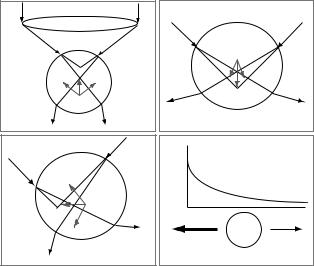
Ashkin and co-workers 1986 description of a single-beam trap presented the necessary requirements for stable trapping of dielectric particles in three dimensions (2). For laser light interacting with a particle of diameter much larger than the laser wavelength, d l, that is the so-called Mie regime, the force on the particle can be calculated using ray optics to determine the momentum transferred from the refracted light to the trapped particle. Figure 1a–c schematically shows the general principle; two representative rays are bent as they pass through the spherical particle producing the forces that push the trapped particle toward the laser focus. A tightly focused beam that is most intense in the center thus pulls the trapped object toward the beam waist. More rigorous treatment and calculations can be found in (2,10).

In the Rayleigh regime, d l, the system must be treated in accordance with wave optics, and again the tight focusing results in a net trapping force due to the fact that the particle is a dielectric in a non-uniform electric field. Figure 1d shows a simplified depiction of force generation in this regime. The electric field gradient from the laser light induces a dipole in the dielectric particle; this results in a force on the particle directed up the gradient toward the area of greatest electric field intensity, at the center of the laser focus. Detailed calculations can be found in Ref. 11.

Position

Figure 2. Relationship between potential, force, and bead position probability. The interaction of the tightly focused laser and dielectric results in a parabolic potential well, the consequence of which is a linear restoring force; the trap behaves as a linear radial spring. Here a positive force pushes the particle to the right. When driven by thermal events in solution a particle’s position has a Gaussian distribution.

practice, theoretical analysis of specific trapping parameters is not necessary because several methods allow direct calibration of trapping forces. Regardless of particle size, a tightly focused laser with a Gaussian intensity profile (TEM00 mode) interacting with a spherical particle, traps the particle in a parabolic potential well. The parabolic potential is convenient because it results in a trap that

behaves like a Hookian spring: restoring force that pushes the particle back toward the focus increases linearly with the displacement from the focus. Figure 2 schematically illustrates the potential well, force profile, and distribution of particle positions for a hypothetical trapped sphere. This convenient relationship results in spherical particles being the natural choice for most trapping applications including gradient. These particles are often referred to as beads, microbeads, or microspheres interchangeably.

Optical Tweezers Systems

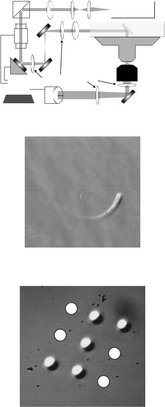
Implementations of optical tweezers as they are applied to biology are variations on a theme: most systems share several common features although details vary and systems are often optimized for the application. Figures 3 and 4 show a photograph and a diagram of an example system. Generally, the system begins with a collimated, plane-polarized laser with excellent power and pointing stability. The optimal laser light wavelength depends on the application, but near-infrared (IR) lasers with a wavelength 1 mm are a typical choice for use with biological samples; such lasers are readily available and biological samples generally exhibit minimal absorption in the near-IR. A light attenuator allows for adjustment of laser power and therefore trap stiffness. In the example system this is accomplished with a variable half-wave plate that adjusts the polarity prior to the beam passing through a polarized beam splitting cube that redirects the unwanted laser power. Most systems then contain a device and lenses to actively steer the beam. In the case of the example system, a piezo-actuated mirror creates angular deflections of the beam that the telescope lenses translate into lateral position changes of the laser focus at the focal plane of the objective. This is accomplished by arranging the telescope so that a virtual image of the steering device is formed at the back aperture of the microscope objective lens. This arrangement also assures that the laser is not differentially clipped by the objective aperture as the trap is steered. Following the steering optics, the laser enters a microscope, is focused by a high numerical

Figure 3. Photograph of an optical tweezers instrument. Note the vibration isolation table that prevents spurious vibrations from affecting experiments. The clear plastic cover minimizes ambient air convection that might affect the laser path in addition to limiting access of dust and preventing accidental contact with the optics.

aperture objective, and encounters the sample. After passing through the trapping/image plane, the laser usually exits the microscope and enters a detection system, which in this case employs back-focal-plane interferometry to measure the position of the bead relative to the trap (14–16).

There are many optical tweezers designs that can produce stable, reliable trapping. In most cases, the system is integrated into an inverted, high quality research microscope (17,18), although successful systems have been incorporated into upright (e.g., 15) or custom built microscopes (14). Some use a single laser to form the trap (7,15) while a more complicated arrangement uses two counterpropagating lasers (19,20).

Various implementations for detecting the bead position include image analysis (21,22), back focal plane interferometry (BFPI) (14,16), and a host of less frequently applied methods based on measurements of scattered or fluorescent light intensity (23–25) or interference between two beams produced using the Wollaston prisms associated with differential interference contrast microscopy (26). Trap steering can be accomplished with acoustooptic deflectors (15,27,28), steerable mirrors (23), or actuated lenses (14). Figure 5 shows a silica microsphere in a trap being moved in a circle at > 10 revolutions s 1 using acoustooptic deflectors, resulting in the comet tail in the image. Alternatively, the sample can be moved with a motorized or piezoactuated nanopositioning stage. In addition, splitting the laser into two orthogonally polarized beams, fast laser steering to effectively multiplex the beam by rapidly jumping the laser between multiple positions (29), or holographic technology (9) can be used to create arrays of multiple traps. Figure 6 shows an image of a 3 3 array of optical traps created using fast beam steering to multiplex a single beam. Five traps are holding beads while four, marked with white circles are empty. Specific optical tweezers designs can also allow incorporation of other advanced optical techniques often used in biology, including, but not limited to, total internal reflection microscopy and confocal microscopy (30).

Figure 5. Micrograph of 1 mm bead being manipulated in a circle with an optical tweezers device. The comet tail is the result of the bead moving faster than the video frame rate.

Figure 6. Micrograph of a 3 3 array of traps produced by time sharing a single laser between nine positions. The traps at the four locations marked with white circles are empty while the other five hold a 1 mm diameter silica microsphere.

Detection

Determining the force on a trapped sphere requires measurement of the displacement of the trapped particle from the center of the optical trap. Back focal plane interferometry (BFPI) is the most popular method, and allows high speed detection with nanometer resolution. Rather than following an image of the bead, which is also a viable detection technique, BFPI tracks the bead by examining how an interference pattern formed by the trapping laser is altered by the bead interacting with the laser further up the beam at the microscope focal plane. This interference pattern is in focus at the back focal plane of the condenser lens of the microscope, thus the name of the technique.

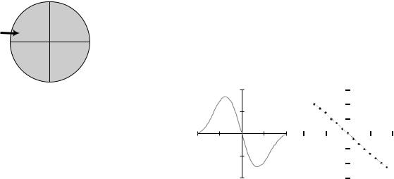
Laser light interacting with the bead is either transmitted or scattered. The transmitted and scattered light interfere with one another resulting in an interference pattern that is strongly dependent on the relative position of the bead within the trap. This interference pattern is easily imaged onto a quadrant photodiode (QPD) detector positioned at an image plane formed conjugate to the back focal plane of the condenser lenes by supplemental lenses (e.g., BFPI imaging lens in Fig. 4). A simple divider-ampli- fier circuit compares the relative intensity in each quadrant according to the equations shown in Fig. 7. This results in voltage signals that follows the position of the bead in the trap.

Back focal plane interferometry has several important advantages compared with the other commonly used bead tracking techniques. Typically, image analysis limits the data collection rate to video frame rate, 30 Hz, or slower if images must be averaged, while BFPI easily achieves sampling frequencies in the tens of kilohertz. Under ideal conditions, image analysis can detect particle positions with 10 nm resolution, while BFPI achieves

Quadrant Photodiode

C D

y

X= (A+C)-(B+D)

A+B+C+D

Y= (A+B)-(C+D)

A+B+C+D

Figure 7. Quadrant photodiode operation. The circular quadrant photodiode detector is composed of four individual detectors (A–D) each making up one quarter of the circle. Each diode measures the light intensity falling on the surface of that quadrant and the associated electronics compares the relative intensities according to the equations shown in the figure. The resulting voltages are calibrated to the intensity shifts caused by the bead as it moves to different positions in the trap.

subnanometer resolution. Speeds and resolution similar to BFPI can be achieved by directly imaging a bead onto a QPD, however, it can be inconvenient in systems where trap steering is employed because the image of the particles will move across the detector as the trap moves in the image plane of the microscope, thus requiring frequent repositioning of the detector. With BFPI, the position of the intereference pattern at the back focal plane of the condenser does not move as the trap is steered, so the detector can remain stationary.

Calibration

Although BFPI provides a signal corresponding to bead position, two important system parameters must be measured before forces and positions can be inferred. The first is the detection sensitivity, b, relating the detector signal to the particle position. The second is the Hookian spring constant, k, where

where x is the displacement of the particle from the center of the trap. Both sensitivity and stiffness depend on the diameter of the particle and the position of the trap relative to nearby surfaces. Stiffness is linear with laser power while sensitivity, when using BFPI, does not depend on laser power as long as the detector is operating in its linear range. Ideally, these parameters are determined in circumstances as near to the experimental conditions as possible. Indeed whenever reasonably possible, it is wise to account for bead and assay variation by determining these parameters for each bead used in an experiment.

Direct Calibration Method

Sensitivity can be measured by two independent methods. The most direct is to move a bead affixed to a coverslip through the laser focus with a nanopositioning piezocontrolled stage, or conversely by scanning the laser over the immobilized bead while measuring the detector signal. An example calibration curve is shown in Fig. 8 for a system using BFPI. The linear region within 150 nm on either side of zero is fit to a line to arrive at the sensitivity, b, equal to 6.8 10 4 V nm 1. The second method is discussed below under calibration with thermally driven motion.

Figure 8. Optical tweezers sensitivity curve acquired with the direct method of moving the laser past an immobilized bead. The full curve is shown in a. The central linear region shown in b is fit to give a sensitivity of 6.8 10 4 V nm 1.

180 OPTICAL TWEEZERS

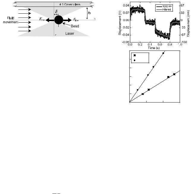
Figure 9. Schematic of drag force calibration. Uniform fluid flow from the left produces a force on the bead that can be calculated with the equations in the text. The bead is displaced to a distance, where the force due to fluid flow is balanced by the force due to the trap.

The direct calibration for sensitivity has the disadvantage of requiring the bead to be immobilized, typically to the coverslip, whereas experiments are typically conducted several microns from the surface. Additionally, with the bead fixed to a surface, its z-axis position is no longer controlled by the trapping forces, resulting in the possibility that the measured sensitivity does not correspond to the actual z axis position of a trapped particle. Estimates of sensitivity may also be rendered inaccurate if attachements to the surface slip or fail. Consequently, thermal force based calibration discussed in the next section are often more reliable.

The trap stiffness, k, can be measured by applying drag force from fluid flow to the trapped particle. Figure 9 shows a schematic representation of the trap, particle, and fluid movement. Typically, a flow is induced around the bead by moving the entire experimental chamber on a motorized or piezodriven microscope stage. In the low Reynolds number regime where optical traps are typically applied, the drag coefficient, g, on a sphere in the vicinity of a surface can be accurately calculated:

where r is the radius of the microsphere, h is the viscosity of the medium, and c is the correction for the distance from a surface given by

where h is the distance from the center of the sphere to the surface. Equation 3 is an approximation and can be carried to higher order for greater accuracy (31).

The force due to fluid flow is readily calculated

where V is the velocity of the particle relative to the fluid medium.

When a flow force is applied to the trapped microsphere, the bead moves away from the center of the trap to an equilibrium position where the flow force and trapping force balance. Applying several drag forces (using a range of fluid flow velocities) and measuring the deflection in each case allows one to plot force of the trap as a function of bead position. The slope of this line is the trap stiffness, k.

0.5

0

Displacement (nm)

Figure 10. Results of a typical drag force calibration. (a) Typical signal of five averaged applications of uniform drag force on a trapped microsphere. In the region labeled 1, the bead quickly achieves a stable displacement due to the constant velocity. In region 2, the bead briefly returns to the center of the trap as the stage stops. In region 3, the bead is again displaced as the stage moves back to its home position and in region 4 the stage is at rest in its home position. The displaced position () in region 1 is averaged to determine the displacement for a given flow force. (b) Example of data from several different forces applied to the trapped microsphere reveal a linear relation to displacement.

Figure 10a shows a trace of a bead being displaced by fluid drag force provided by a piezoactuated stage moving at a known velocity. In the first region the bead quickly achieves and holds a stable position as long as the stage moves at a constant velocity, making measurement of the displacement relatively simple. When the stage stops the bead returns to the center of the trap as is seen in the second section of the record. The subsequent negative deflection in the third section is the result of the stage returning to its original position at a non-uniform speed. Figure 10b shows force as a function of position for two laser powers; the linear fitting coefficient gives the trap stiffness in each case.

In practice, calibration by viscous drag can be quite labor intensive, and the requirement for the sample to be moved repeatedly and rapidly is too disruptive to be performed ‘‘on the fly’’ during many types of experiments. A more efficient and less disruptive alternative relies on the fact that the thermal motion of the fluid molecules exerts significant, statistically predictable forces on the trapped microsphere; these result in fluctuations in bead position measurable with the optical tweezers.

Thermal Force Based Calibration Methods

At low Reynold’s (Re) number the power spectrum of the position of a particle trapped in a harmonic potential well subject only to thermal forces takes the form of a Lorentzian (32):

where kB is the Boltzmann constant, f is the frequency, fc is a constant called the corner frequency, and

There are several important practical considerations for applying the power spectrum to calibrate optical tweezers. The mathematical form of the power spectrum does not account for the electrical noise in the signal, so a large signal to noise ratio is required for accurate calibration. In addition, records of bead position must be treated carefully, especially with respect to instrument bandwidth and vibrations, to yield the correct shape and magnitude of the power spectrum.

A typical calibration begins by setting the position of the bead relative to any nearby surface, typically a microscope sample coverglass. With the bead positioned, a record of thermal motion of the bead is taken. For the example system in Figs. 3 and 4 a typical data collection for a calibration is 45 s at maximum bandwidth of the QPD and associated electronics. The data is then low pass (antialias) filtered using a high order Butterworth filter with a cut-off frequency set to one-half of the bandwidth.

Following acquisition and filtering, the power spectrum of the record of bead position is calculated. In practice, many power spectra should be averaged to reduce the inherently large variance of an individual power spectrum. For example, the 45 s of data is broken into 45, 1 s records of bead position, the power spectrum for each is calculated and the spectra are averaged together. To accurately compute the power spectrum the data must be treated as continuous; this is achieved by wrapping the end of the record back to meet the beginning. To avoid a discontinuity where the beginning and end are joined, each record is windowed with a triangle or similar function that forces the ends to meet but maintains the statistical variance in the original record. Figure 11a shows an example of an averaged power spectrum. Note the units on the y axis: often, power spectra are presented in different units according to their intended use. Accurate calibration of optical tweezers requires that the power spectrum be in nm2 Hz 1 or, provided volts are proportional to displacement, V2 Hz 1.

The average power spectrum is expected to fit the form of equation 5. To avoid aliased high frequency data corrupting the fit to the power spectrum, the spectrum is cropped well below the cut-off frequency of the antialiasing

Slope = 4.4x10–4pN/nm/mW

(b)

Figure 11. Example power spectrum calibration. (a) An example power spectrum (gray) and Lorentzian fit (black). (b) Power spectrum calibrations for five separate laser powers showing the linear dependence of stiffness on laser power.

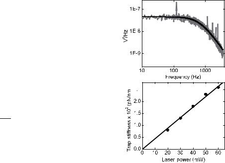
filter. The average, cropped power spectrum can be visually inspected for evidence of noise (e.g., spikes or other deviations from the expected Lorentzian form) and fit to equation 5, with fc and B as fitting parameters. The drag coefficient is calculated using equations 2 and 3 and the stiffness, k, is then calculated with a simple rearrangement of equation 7. The sensitivity, b, can also be calculated by recognizing that the value of B produced by the fit is proportional to the signal power. The value of B can be calculated from first principles by applying equation 6. In practice, the value of B is determined by fitting equation 5 with B as a parameter. Equation 6 gives B in units of nm2 Hz 1 while the fitted value of B will typically be V2 Hz 1. The parameter b is then determined by dividing the fitted value by the theoretical value and taking the square root. Figure 11b shows an example power spectrum used to calculate the trap stiffness and the sensitivity of the detection system with a 0.6 mm bead.

Inspection of the power spectrum in Fig. 11a shows two distinct regions: the low frequency plateau and the high frequency roll off. These two sections can be qualitatively understood as representing two aspects of the motion of the trapped particle. The high frequency roll-off is representative of small, rapid oscillations of the bead in the trap. Since the distance the bead moves over these short time scales is generally small, the bead does not ‘‘feel’’ large changes in the force of the trap pushing it back to the center, and hence this motion has the character of free diffusion. At lower frequency, the spectrum is flat, because large-scale oscillations are attenuated by the trap pushing the bead back to the center. As a result low frequency oscillations do not exhibit the character of free diffusion; the bead feels the trap when it makes a large excursion.

182 OPTICAL TWEEZERS

The methods for calculating and then fitting the power spectrum above are adequate in most cases and for most experiments. However, several additional considerations can be added to this relatively simple approach to improve the accuracy in some situations. These include, but are not limited to, accounting for the frequency dependence of the drag coefficient, and theoretically accounting for aliasing that may be present in the signal (54).

Two other calibration methods also take advantage of thermal forces acting on trapped beads. These methods are not conceptually distinct from the power spectrum method, but treat the data differently, are susceptible to different errors, and thus provide a good cross-check with the power spectrum and direct methods above.

As one would expect, the range of bead position should decrease with increasing trap stiffness. For an overdamped harmonic potential, such as a spherical bead in an optical trap, this relation has a specific mathematical form:

considering the drag coefficient altogether, but this method relies on accurate estimation of the sensitivity squared (b2). Furthermore, the variance method can lead to inaccurate stiffness measurements because system drift will inflate the variance, leading to underestimated trap stiffness.

A safe course is to (1) inspect the power spectrum for evidence of external noise, (2) calculate the stiffness and sensitivity by fitting the power spectrum, (3) recalculate the stiffness with the variance method using the sensitivity determined from the power spectrum, and (4) compare the stiffness results from each method. If the stiffness agrees between the two it indicates that the drag coefficient and sensitivity are both correct. The only possibility for error would be that they are both in error in a manner that is exactly offsetting, which is quite unlikely. Comparison with the direct manipulation methods can alleviate this concern.

tweezers were being applied to biological measurements (2,7). In the years that followed, optical tweezers became increasingly sophisticated, and their contributions to biology and biophysics in particular grew rapidly. Some important experimental considerations, and contributions to basic science made possible by optical tweezers, highlighted representative assays, and results are discussed in this section.

Practical Experimental Concerns

Beyond the design and calibration challenges, there are additional concerns that come into play preparing an experimental assay for use with optical tweezers. The most general of these attached is a trappable object to the system being studied, and accounting for series compliances when interpreting displacements of this object.

Probably the most popular attachment scheme currently in use is the biotin-streptavidin linkage. Microbeads are coated with streptavidin, and the structure to be studied, if a protein, can be easily functionalized with biotin via a succinimidyl ester or other chemical crosslinker. When mixed, the streptavidin on the bead tightly binds to biotin on the structure to be studied. Beads coated in this manner tend to stick to the surfaces in the experimental chamber, which is inconvenient for setting up an experiment, and recently developed neutravidin is an attractive alternative to streptavidin with decreased nonspecific binding at close to neutral pH. Alternative attachment schemes usually involve coating the bead with a protein that specifically interacts with the structure to be studied. For example, a microtubule-associated protein might be attached to the bead; subsequently that bead sticks to microtubules, which can then be manipulated with the optical tweezers. Recombinant DNA technology can also be used; in this case the amino acid sequence of a protein is modified to add a particular residue (e.g., reactive cystein), which serves as a target for specific crosslinking to the bead. This approach provides additional control over the binding orientation of the protein, but runs the risk that the recombinant protein many not behave as the wild type.

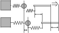
Interpreting displacements measured with optical tweezers is complicated by compliances in the system under study, or the linkage to the trapped bead; these must be accounted for to determine the actual displacement of specific elements. Figure 12 diagrams the compliances in a sample system. A filament to which the trapped bead is linked is pulled to the right by the force generating process under study (not shown). This causes the bead to be displaced to the right within the trap by an amount, D Bead, which is directly measured. However, the other compliance

in the system, klinkage, is also stretched and takes up some amount of the filament displacement, which can only be

determined with knowledge of the link stiffness; thus the measured displacement is less than the actual displacement of the filament. In some situations it may be possible to measure the link stiffness directly, but generally this is not possible during an experiment. Furthermore, the link stiffness is usually nonlinear, and may be complicated by

Figure 12. Schematic diagram of series compliances in optical tweezers experiments. Both the optical trap and the linkage between the bead and hypothetical filament are shown as springs. The optical trap is a well characterized spring, having been carefully calibrated prior to beginning experiments. The stiffness of the linkage, however, is unknown. When the filament is pulled to the right by a hypothetical motor or other biological system, both springs are stretched. Therefore the displacement of the trapped bead is not necessarily equal to the displacement of the filament by the motor. Examination of the system shows that the force on the trapped bead is the same as the force on the filament once all elements have reached their equilibrium. Knowledge of klinkage would allow for displacements at the bead to be used to calculate filament displacements.

the bead rocking about the link under forces applied by the trap. When precision displacement measurements are desired these difficulties can be circumvented with a feedback system that maintains a constant force on the particle (force clamp). By maintaining constant force, the link is held at a fixed strain and the movements of the feedback controlled laser directly follow the positional changes of the filament.

Motor Proteins: Kinesin And Myosin

The kinesins and myosins are two large families of motor proteins that convert chemical energy released by adenosine triphosphate (ATP) hydrolysis into mechanical work. Kinesins move cargo along microtubules while myosins exert forces against actin filaments, most notably in muscle. Many of the mechanical and kinetic aspects of these molecules behaviors have been determined from measurements made with optical tweezers. These include the length of displacements during individual chemomechanical steps, single molecule force generation capabilities, and kinetic information about the enzymatic cycle that converts chemical into mechanical energy.

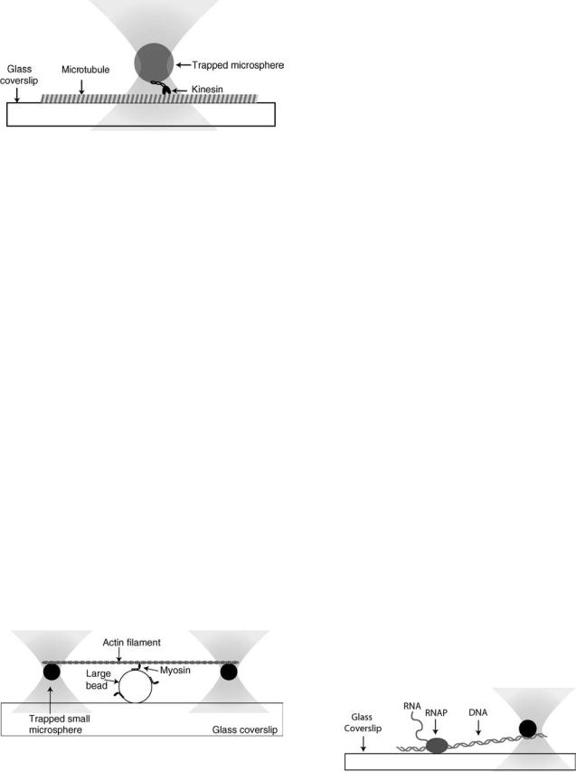
Due to the differences in the substrate along which myosin and kinesin motors move, and the nature of their movements, assays for studying them have significantly different geometries. In the case of kinesin (Fig. 13), generally a single bead coated with the motor is held in an optical trap (17,26). The motors are sparsely coated on the beads, so that only one motor interacts with the microtubule track, which has been immobilized onto a glass surface. The optical tweezers manipulate the coated bead onto the microtubule; bead movements ensue when a kinesin motor engages the microtubule lattice. If the

184 OPTICAL TWEEZERS

Figure 13. Schematic of an experiment to study kinesin. The motor protein kinesin is processive, meaning that the motor spends a large portion of its force generating cycle attached to the microtubule and is able to maintain movement when only a single motor is present. As a result, a single, sparsely coated bead held in an optical trap can be used to measure the force generating properties of kinesin.

optical tweezers are used in stationary mode, the records will indicate a fraction of the actual motor displacement, the remainder being taken up in the compliant link between the bead and the motor as described above. The actual displacements of the motor must then be inferred using estimates of the bead-motor link compliance, which is estimated in independent experiments (26).

Alternatively, a force clamp is applied to adjust the position of the trap to maintain a constant force on the bead as the kinesin motor travels along the microtubule. The movement of the motor is then inferred from the adjustments to the laser position, which directly reveal 8 nm steps, demonstrating that the kinesin molecule moves along the microtubule with the same periodicity as the microtubule lattice. Additional analysis of this data showed that kinesin stalls under loads of 5–8 pN, dependent on ATP concentration, and exhibits tight coupling between ATP hydrolysis and force generation (17,34).

Assays for studying myosin (Fig. 14) are somewhat more complicated, relying on two traps, each holding a microsphere, and a third large bead sparsely coated with myosin affixed to the surface of the microscope slide (35). An actin filament strung between the two smaller microspheres, each held by separate traps, is lowered into a

position where myosin on the large fixed bead can pull against it. Myosin is not processive; it spends only a small fraction of the force generating cycle attached to the actin filament, and an unrestrained filament will diffuse away from the motor during the detached portion of the cycle. Thus the filament is held in close contact with the motor to allow repeated force generating interactions to be observed.

The actin filament and attached beads will move back and forth due to Brownian motion, which is limited by the drag on the particle and the force provided by the trap. This has two important consequences: the myosin molecule on the large bead is exposed to a number of possible binding sites along the actin filament, and attachment of the myosin cross bridge elevates the stiffness of the system sufficiently to greatly reduce the extent of thermally induced bead motion. With bandwidth sufficient to detect the full extent of microsphere Brownian motion, myosin binding events are identified by the reduction in the amplitude of the thermal motion. The distribution of positions of the trapped microspheres and filament at the onset of binding events is expected to be Gaussian of the same width as if the myosin-coated bead was absent. However, shortly after binding, the myosin motor displaces the filament and this shifts the center of the Gaussian by the distance of a single myosin step. Analysis of high resolution, high bandwidth traces of bead position with the above understanding lead to determination of the step length for single myosin subfragment-1 and heavy meromyosin: 3.5 and 5 nm, respectively (28).

Other Motor Proteins

In addition to the classic motor proteins that generate forces against cytoskeletal filaments, proteins may exhibit motor activity, not as their raison d’etre, but in order to achieve other enzymatic tasks. One such protein is ribonucleic acid (RNA) polymerase (RNAP), the enzyme responsible for transcription of genetic information from deoxyribonucleic acid (DNA) to RNA. The RNAP uses the energy of ATP hydrolysis to move along the DNA substrate, copying the genetic information at a rate of 10 base pairs per second. The movement is directed, and thus constitutes motor activity. The assay used to study RNAP powered movement along the DNA substrate is shown in Fig. 15. A piece of single-stranded DNA attached to the trapped glass microsphere is allowed to interact with an RNAP molecule affixed to the surface of the slide. Optical tweezers hold the bead so that the progress and force developed by RNAP can be monitored. As the RNAP molecule moves along the

DNA, the load opposing the motor movement increases until the molecule stalls (36,37). Details of the kinetics of RNAP can be inferred from the relation between the force and speed of movement.

Nonstandard Trapping

A number of research efforts have studied the trapping of nonspherical objects and/or applied them to study biological processes. For example, the stiffness of a microtubule was measured using optical tweezers to directly trap and bend the rod-like polymer. Image data of the induced microtubule shape were then used in conjunction with mechanical elastic theory to determine the stiffness of the microtubule (38). Recently, there has been significant interest in using optical traps to exert torques. Generally, these techniques rely on nonspherical particles, non-Gaussian beams, or birefringent particles to create the necessary asymmetry to develop torque. One approach relies on using an annular laser profile (donut mode) with an interfering reference beam to create a trapping beam that has rotating arms (39). With such an arrangement torque generation is not dependent on the particle shape, but the implementation is relatively complicated. Two closely located traps can also be used to rotate objects by trapping them in multiple locations and moving the traps relative to one another. Using a spatial light modulator, which splits the beam into an arbitrary number of individual beams, to create and move the two traps allows rotation about an axis of choice (40).

For experimental applications, it is generally desirable to calibrate the torque exerted on the particles. The above techniques are not easily calibrated. A more readily calibrated altenative uses birefringent particles such as quartz microspheres (41). The anisotropic polarizability of the particle causes it to align to the beam polarity vector. The primary advantage of this technique is that the drag coefficient of the spherical particle is easily calculated, allowing torques can be calibrated by following rotational thermal motion of the particle, similarly to the techniques described for thermal motion calibrations above.

Modulation of trap position along with laser power or beam profile can create a laser line trap (42–44). The scheme is similar to time sharing a single laser between several positions to create several traps. However, to form a line trap the laser focus is rapidly scanned through positions along a single line. With simultaneous power modulation a linear trapping region capable of applying a single constant force to a trapped particle along the entire length of the trap is created. This technique can be used to replace the conventional force clamp relying on electronic feedback.

Some Other Optical Tweezers Assays

Optical tweezers have made numerous contributions to other subfields. A number of groups have utilized optical tweezers to study DNA molecules. Stretching assays have produced force extension relations for purified DNA, and stretching of individual nucleosomes revealed sudden drops in force indicative of the opening of the coiled DNA structure (45). Optical trapping has also been used to directly study the forces involved in packaging DNA into

a viral capsid. Packaging was able to proceed against forces > 40 pN, and the force necessary to stall packaging was dependent on the how much of the DNA was already packaged into the capsid (46). Double-stranded DNA has also been melted (unzipped) by pulling the strands apart with optical tweezers: this established that lamba phage (a bacterial virus) DNA unzips and rezips in the range of 10– 15 pN, dependent on the nucleotide sequence (47). Stretching RNA molecules to unfold loops and other secondary structures with a similar assay has been used to test a general statistical mechanics result known as the Jarzinsky Inequality (48).

Similar stretching experiments have been performed on proteins. A good example is the large muscle protein titin, which mediates muscle elasticity. Optical tweezers were applied to repeatedly stretch the molecule, providing evidence of mechanical fatigue of the titin molecule that could be the source of mechanical fatigue in repeatedly stimulated muscles (49).

Experiments that study interactions in larger, more complex systems are increasing common. Microtubules associated to mitotic chromosome kinetochores have been studied with optical tweezers. Forces of 15 pN were generally found to be insufficient to detach kinetochore bound microtubules and kinetochore attachment was found to modify microtubule growth and shortening (21). A number of studies have also applied optical tweezers to study structures inside intact cells and the force generating ability of highly motile cells such as sperm (6,50).

Beyond biological measurements, optical tweezers have utility in assembling micron scale objects in desired positions. Weakly focused lasers operating similarly to optical tweezers have been used to directly pattern multiple cell types on a surface for tissue engineering (55). Optical trapping has also been used for assembly and organization of nonbiological devices, such as groups of particles (51) and 3D structures, such as a crystal lattice (52).

Additionally, optical tweezers have been applied to great advantage in material and physical sciences. A substantial body of work has applied optical tweezers to study colloidal solutions and microrheology (53).

BIBLIOGRAPHY

1.Ashkin A. Acceleration and trapping of particles by radiation pressure. Phys Rev Lett 1970;24:156–159.

2.Ashkin A, Dziedzic JM, Bjorkholm JE, Chu S. Observation of a single-beam gradient force optical trap for dielectric particles. Opt Lett 1986;11:288–290.

3.Ashkin A, Dziedzic JM, Yamane T. Optical trapping and manipulation of single cells using infrared laser beams. Nature (London) 1987;330:769–771.

4.Ashkin A, Dziedzic JM. Optical trapping and manipulation of viruses and bacteria. Science 1987;235:1517–1520.

5.Block SM, Blair DF, Berg HC. Compliance of bacterial flagella measured with optical tweezers. Nature (London) 1989; 338:514–518.

6.Tadir Y, et al. Micromanipulation of sperm by a laser generated optical trap. Fertility Sterility 1989;52:870–873.

7.Block SM, Goldstein LS, Schnapp BJ. Bead movement by single kinesin molecules studied with optical tweezers. Nature (London) 1990;348:348–352.

186 OPTICAL TWEEZERS

8.Grover SC, Skirtach AG, Gauthier RC, Grover CP. Automated single-cell sorting system based on optical trapping. J Biomed Opt 2001;6:14–22.

9.Leach J, et al. 3D manipulation of particles into crystal structures using holographic optical tweezers. Opt Express 2004;12:220–226.

10.Ashkin A. Forces of a single-beam gradient laser trap on a dielectric sphere in the ray optics regime. Biophys J 1992;61: 569–582.

11.Visscher K, Brakenhoff G, Lindmo T, Brevik I. Theroretical study of optically induced forces on spherical particles in a single beam trap I: Rayleigh scatters. Optik 1992;89:174–180.

12.Nahmias YK, Odde DJ. A dimensionless parameter for escape force calculation and general design of radiation force-based systems such as laser trapping and laser guidance. Biophys J 2002;82:166A.

13.Nahmias YK, Gao BZ, Odde DJ. Dimensionless parameters for the design of optical traps and laser guidance systems. Appl Opt 2004;43:3999–4006.

14.Allersma MW, et al. Two-dimensional tracking of ncd motility by back focal plane interferometry. Biophys J 1998;74:1074– 1085.

15.Brouhard GJ, Schek HT, Hunt AJ. Advanced optical tweezers for the study of cellular and molecular biomechanics. IEEE Trans Biomed Eng 2003;50:121–125.

16.Gittes F, Schmidt C. Interference model for back-focal-plane displacement detection in optical tweezers. Opt Lett 1998a;23:7–9.

17.Visscher K, Schnitzer MJ, Block SM. Single kinesin molecules studied with a molecular force clamp. Nature (London) 1999;400:184–189.

18.Ruff C, et al. Single-molecule tracking of myosins with genetically engineered amplifier domains. Nature Struct Bio 2001;8: 226–229.

19.Guck J, et al. The optical stretcher: A novel laser tool to micromanipulate cells. Biophys J 2001;81:767–784.

20.Smith SB, Cui YJ, Bustamante C. Overstretching B-DNA: The elastic response of individual double-stranded and singlestranded DNA molecules. Science 1996;271:795–799.

21.Hunt AJ, McIntosh JR. The dynamic behavior of individual microtubules associated with chromosomes in vitro. Mol Biol Cell 1998;9:2857–2871.

22.Kuo SC, Sheetz MP. Force of single kinesin molecules measured with optical tweezers. Science 1993;260:232–234.

23.Florin EL, Pralle A, Horber JKH, Stelzer EHK. Photonic force microscope based on optical tweezers and two-photon excitation for biological applications. J Struct Biol 1997;119:202– 211.

24.Friese M, Rubinsztein-Dunlop H, Heckenberg N, Dearden E. Determination of the force constant of a single-beam gradient trap by measurement of backscattered light. Appl Opt 1996;35:7112–7116.

25.Pralle A, et al. Three-dimensional high-resolution particle tracking for optical tweezers by forward scattered light. Microsc Res 1999;44:378–386.

26.Svoboda K, Schmidt CF, Schnapp BJ, Block SM. Direct observation of kinesin stepping by optical trapping interferometry. Nature 1993;365:721–727.

27.Lang MJ, Asbury CL, Shaevitz JW, Block SM. An automated two-dimensional optical force clamp for single molecule studies. Biophys J 2002;83:491–501.

28.Molloy JE, et al. Movement and force produced by a single myosin head. Nature (London) 1995;378:209–212.

29.Visscher K, Brakenhoff GJ, Krol JJ. Micromanipulation by multiple optical traps created by a single fast scanning trap integrated with the bilateral confocal scanning laser microscope. Cytometry 1993;14:105–114.

30.Gensch T, et al. Transmission and confocal fluorescence microscopy and time-resolved fluorescence spectroscopy combined with a laser trap: Investigation of optically trapped block copolymer micelles. J Phys Chem B 1998;102:8440–8451.

31.Happel J, Brenner H. Low Reynolds number hydrodynamics. With special applications to particulate media. Leiden: Noordhoff International Publishing; 1973.

32.Gittes F, Schmidt C. Thermal noise limitations on micromechanical experiments. Eur Biophys J with Biophys Lett 1998b;27:75–81.

33.Meiners JC, Quake SR. Direct measurement of hydrodynamic cross correlations between two particles in an external potential. Phy Rev Lett 1999;82:2211–2214.

34.Schnitzer MJ, Block SM. Kinesin hydrolyses one ATP per 8-nm step. Nature (London) 1997;388:386–390.

35.Finer JT, Simmons RM, Spudich JA. Single myosin molecule mechanics - piconewton forces and nanometer steps. Nature (London) 1994;368:113–119.

36.Wang MD, et al. Force and velocity measured for single molecules of RNA polymerase. Science 1998;282:902–907.

37.Yin H, et al. Transcription against an applied force. Science 1995;270:1653–1657.

38.Felgner H, Frank R, Schliwa M. Flexural rigidity of microtubules measured with the use of optical tweezers. J Cell Sci 1996;109(Pt 2):509–516.

39.Paterson L, et al. Controlled rotation of optically trapped microscopic particles. Science 2001;292:912–914.

40.Bingelyte V, Leach J, Courtial J, Padgett MJ. Optically controlled three-dimensional rotation of microscopic objects. Appl Phys Lett 2003;82:829–831.

41.La Porta A, Wang MD. Optical torque wrench: Angular trapping, rotation, and torque detection of quartz microparticles. Phy Rev Lett 2004; 92.

42.Liesfeld B, Nambiar R, Meiners JC. Particle transport in asymmetric scanning-line optical tweezers. Phy Rev 2003; 68.

43.Nambiar R, Meiners JC. Fast position measurements with scanning line optical tweezers. Opt Lett 2002;27:836–838.

44.Nambiar R, Gajraj A, Meiners JC. All-optical constant-force laser tweezers. Bio J 2004;87:1972–1980.

45.Bennink ML, et al. Unfolding individual nucleosomes by stretching single chromatin fibers with optical tweezers. Nature Struct Biol 2001;8:606–610.

46.Smith DE, et al. The bacteriophage phi 29 portal motor can package DNA against a large internal force. Nature (London) 2001;413:748–752.

47.Bockelmann UP, et al. Unzipping DNA with optical tweezers: high sequence sensitivity and force flips. Biophys J 2000; 82:1537–1553.

48.Liphardt J, et al. Equilibrium information from nonequilibrium measurements in an experimental test of Jarzynski’s equality. Science 2002;296:1832–1835.

49.Kellermayer MS, Smith SB, Granzier HL, Bustamante C. Folding-unfolding transitions in single titin molecules characterized with laser tweezers. Science 1997;276:1112– 1116.

50.Aufderheide KJ, Du Q, Fry ES. Directed positioning of micronuclei in paramecium-tetraurelia with laser tweezers— absence of detectable damage after manipulation. J Eukaryotic Microbiol 1993;40:793–796.

51.Misawa H, et al. Multibeam laser manipulation and fixation of microparticles. Appl Phys Lett 1992;60:310–312.

52.Holmlin RE, et al. Light-driven microfabrication: Assembly of multicomponent, three-dimensional structures by using optical tweezers. Angew Chem Int Ed Engl 2000;39:3503–3506.

53.Lang MJ, Block SM. Resource letter: LBOT-1: Laser-based optical tweezers. Am J Phy 2003;71:201–215.