

- •VOLUME 5
- •CONTRIBUTOR LIST
- •PREFACE
- •LIST OF ARTICLES
- •ABBREVIATIONS AND ACRONYMS
- •CONVERSION FACTORS AND UNIT SYMBOLS
- •NANOPARTICLES
- •NEONATAL MONITORING
- •NERVE CONDUCTION STUDIES.
- •NEUROLOGICAL MONITORS
- •NEUROMUSCULAR STIMULATION.
- •NEUTRON ACTIVATION ANALYSIS
- •NEUTRON BEAM THERAPY
- •NEUROSTIMULATION.
- •NONIONIZING RADIATION, BIOLOGICAL EFFECTS OF
- •NUCLEAR MAGNETIC RESONANCE SPECTROSCOPY
- •NUCLEAR MEDICINE INSTRUMENTATION
- •NUCLEAR MEDICINE, COMPUTERS IN
- •NUTRITION, PARENTERAL
- •NYSTAGMOGRAPHY.
- •OCULAR FUNDUS REFLECTOMETRY
- •OCULAR MOTILITY RECORDING AND NYSTAGMUS
- •OCULOGRAPHY.
- •OFFICE AUTOMATION SYSTEMS
- •OPTICAL FIBERS IN MEDICINE.
- •OPTICAL SENSORS
- •OPTICAL TWEEZERS
- •ORAL CONTRACEPTIVES.
- •ORTHOPEDIC DEVICES MATERIALS AND DESIGN OF
- •ORTHOPEDICS PROSTHESIS FIXATION FOR
- •ORTHOTICS.
- •OSTEOPOROSIS.
- •OVULATION, DETECTION OF.
- •OXYGEN ANALYZERS
- •OXYGEN SENSORS
- •OXYGEN TOXICITY.
- •PACEMAKERS
- •PAIN SYNDROMES.
- •PANCREAS, ARTIFICIAL
- •PARENTERAL NUTRITION.
- •PERINATAL MONITORING.
- •PERIPHERAL VASCULAR NONINVASIVE MEASUREMENTS
- •PET SCAN.
- •PHANTOM MATERIALS IN RADIOLOGY
- •PHARMACOKINETICS AND PHARMACODYNAMICS
- •PHONOCARDIOGRAPHY
- •PHOTOTHERAPY.
- •PHOTOGRAPHY, MEDICAL
- •PHYSIOLOGICAL SYSTEMS MODELING
- •PICTURE ARCHIVING AND COMMUNICATION SYSTEMS
- •PIEZOELECTRIC SENSORS
- •PLETHYSMOGRAPHY.
- •PNEUMATIC ANTISHOCK GARMENT.
- •PNEUMOTACHOMETERS
- •POLYMERASE CHAIN REACTION
- •POLYMERIC MATERIALS
- •POLYMERS.
- •PRODUCT LIABILITY.
- •PROSTHESES, VISUAL.
- •PROSTHESIS FIXATION, ORTHOPEDIC.
- •POROUS MATERIALS FOR BIOLOGICAL APPLICATIONS
- •POSITRON EMISSION TOMOGRAPHY
- •PROSTATE SEED IMPLANTS
- •PTCA.
- •PULMONARY MECHANICS.
- •PULMONARY PHYSIOLOGY
- •PUMPS, INFUSION.
- •QUALITY CONTROL, X-RAY.
- •QUALITY-OF-LIFE MEASURES, CLINICAL SIGNIFICANCE OF
- •RADIATION DETECTORS.
- •RADIATION DOSIMETRY FOR ONCOLOGY
- •RADIATION DOSIMETRY, THREE-DIMENSIONAL
- •RADIATION, EFFECTS OF.
- •RADIATION PROTECTION INSTRUMENTATION
- •RADIATION THERAPY, INTENSITY MODULATED
- •RADIATION THERAPY SIMULATOR
- •RADIATION THERAPY TREATMENT PLANNING, MONTE CARLO CALCULATIONS IN
- •RADIATION THERAPY, QUALITY ASSURANCE IN
- •RADIATION, ULTRAVIOLET.
- •RADIOACTIVE DECAY.
- •RADIOACTIVE SEED IMPLANTATION.
- •RADIOIMMUNODETECTION.
- •RADIOISOTOPE IMAGING EQUIPMENT.
- •RADIOLOGY INFORMATION SYSTEMS
- •RADIOLOGY, PHANTOM MATERIALS.
- •RADIOMETRY.
- •RADIONUCLIDE PRODUCTION AND RADIOACTIVE DECAY
- •RADIOPHARMACEUTICAL DOSIMETRY
- •RADIOSURGERY, STEREOTACTIC
- •RADIOTHERAPY ACCESSORIES
234 PERIPHERAL VASCULAR NONINVASIVE MEASUREMENTS
80.Canonico V, et al. Evaluation of a feedback model based on simulated interstitial glucose for continuous insulin infusion. Diabetologia 2002;45(Suppl. 2):995.
81.Bode B, et al. Alarms based on real-time sensor glucose values alert patients to hypoand hyperglycemia: the guardian continuous monitoring system. Diabetes Technol Ther 2004; 6:105–113.
82.Chassin LJ, Wilinska ME, Hovorka R. Evaluation of glucose controllers in virtual environment: Methodology and sample application. Artif Intell Med 2004;32:171–181.
83.Van den Berghe G, et al. Intensive insulin therapy in the surgical intensive care unit. N Engl J Med 2001;345:1359– 1367.
84.Hogan P, Dall T, Nikolov P. Economic costs of diabetes in the US in 2002. Diabetes Care 2003;26:917–932.
See also GLUCOSE SENSOR; HEART, ARTIFICIAL.
PARENTERAL NUTRITION. See NUTRITION,
PARENTERAL.
PCR. See POLYMERASE CHAIN REACTION.
PERCUTANEOUS TRANSLUMINAL CORONARY
ANGIOPLASTY. See CORONARY ANGIOPLASTY AND GUIDEWIRE DIAGNOSTICS.
PERINATAL MONITORING. See FETAL MONITORING.
PERIPHERAL VASCULAR NONINVASIVE MEASUREMENTS
CHRISTOPH H. SCHMITZ
HARRY L. GRABER
RANDALL L. BARBOUR
State University of New York
Brooklyn, New York
INTRODUCTION
The primary task of the peripheral vasculature (PV) is to supply the organs and extremities with blood, which delivers oxygen and nutrients, and to remove metabolic waste products. In addition, peripheral perfusion provides the basis of local immune response, such as wound healing and inflammation, and furthermore plays an important role in the regulation of body temperature. To adequately serve its many purposes, blood flow in the PV needs to be under constant tight regulation, both on a systemic level through nervous and hormonal control, as well as by local factors, such as metabolic tissue demand and hydrodynamic parameters. As a matter of fact, the body does not retain sufficient blood volume to fill the entire vascular space, and only 25% of the capillary bed is in use during resting state. The importance of microvascular control is clearly illustrated by the disastrous effects of uncontrolled blood pooling in the extremities, such as occurring during certain types of shock.
Peripheral vascular disease (PVD) is the general name for a host of pathologic conditions of disturbed PV function.
Peripheral vascular disease includes occlusive diseases of the arteries and the veins. An example is peripheral arterial occlusive disease (PAOD), which is the result of a buildup of plaque on the inside of the arterial walls, inhibiting proper blood supply to the organs. Symptoms include pain and cramping in extremities, as well as fatigue; ultimately, PAOD threatens limb vitality. The PAOD is often indicative of atherosclerosis of the heart and brain, and is therefore associated with an increased risk of myocardial infarction or cerebrovascular accident (stroke).
Venous occlusive disease is the forming of blood clots in the veins, usually in the legs. Clots pose a risk of breaking free and traveling toward the lungs, where they can cause pulmonary embolism. In the legs, thromboses interfere with the functioning of the venous valves, causing blood pooling in the leg (postthrombotic syndrome) that leads to swelling and pain.
Other causes of disturbances in peripheral perfusion include pathologies of the autoregulation of the microvasculature, such as in Reynaud’s disease or as a result of diabetes.
To monitor vascular function, and to diagnose and monitor PVD, it is important to be able to measure and evaluate basic vascular parameters, such as arterial and venous blood flow, arterial blood pressure, and vascular compliance.
Many peripheral vascular parameters can be assessed with invasive or minimally invasive procedures. Examples are the use of arterial catheters for blood pressure monitoring and the use of contrast agents in vascular X ray imaging for the detection of blood clots. Although they are sensitive and accurate, invasive methods tend to be more cumbersome to use, and they generally bear a greater risk of adverse effects compared to noninvasive techniques. These factors, in combination with their usually higher cost, limit the use of invasive techniques as screening tools. Another drawback is their restricted use in clinical research because of ethical considerations. Although many of the drawbacks of invasive techniques are overcome by noninvasive methods, the latter typically are more challenging because they are indirect measures, that is, they rely on external measurements to deduce internal physiologic parameters. Noninvasive techniques often make use of physical and physiologic models, and one has to be mindful of imperfections in the measurements and the models, and their impact on the accuracy of results. Noninvasive methods therefore require careful validation and comparison to accepted, direct measures, which is the reason why these methods typically undergo long development cycles.
Even though the genesis of many noninvasive techniques reaches back as far as the late nineteenth century, it was the technological advances of the second half of the twentieth century in such fields as micromechanics, microelectronics, and computing technology that led to the development of practical implementations. The field of noninvasive vascular measurements has undergone a developmental explosion over the last two decades, and it is still very much a field of ongoing research and development.
This article describes the most important and most frequently used methods for noninvasive assessment of
the PV; with the exception of ultrasound techniques, these are not imaging-based modalities. The first part of this article, gives a background and introduction for each of these measuring techniques, followed by a technical description of the underlying measuring principles and technical implementation. Each section closes with examples of clinical applications and commercially available systems. The second part of the article briefly discusses applications of modern imaging methods in cardiovascular evaluation. Even though some of these methods are not strictly noninvasive because they require use of radioactive markers or contrast agents, the description is meant to provide the reader with a perspective of methods that are currently available or under development.
NONIMAGING METHODS
Arterial Blood Pressure Measurement
Arterial blood pressure (BP) is one of the most important cardiovascular parameters. Long-term monitoring of BP is used for the detection and management of chronic hypertension, which is a known major risk factor for heart disease. In this case, it is appropriate to obtain the instantaneous BP at certain intervals, such as days, weeks, or months, because of the slow progression of the disease.
In an acute care situation, such as during surgery or in intensive care, continuous BP measurements are desired to monitor heart function of the patients. The following sections describe the most important techniques.
Instantaneous BP Measurements
The most widely used approach is the auscultatory method, or method of Korotkoff, a Russian military physician, who developed the measurement in 1905. A pressure cuff is inflated to 30 mmHg (3.99 k Pa) above systolic pressure on the upper extremity. While subsequently deflating the cuff at a rate of 2 (0.26)–3 mmHg (0.39 kPa) (1), the operator uses a stethoscope to listen to arterial sounds that indicate the points at which cuff pressure equals the systolic and diastolic pressure. The first is indicated by appearance of a ‘‘tapping’’ sound, while the latter is identified by the change from a muffled to vanishing sound.
A second widespread BP measurement technique is the oscillatory method. Here, the cuff contains a pressure sensor that is capable of measuring cuff pressure oscillations induced by the arterial pulse. The cuff is first inflated to achieve arterial occlusion, and then deflated at rate similar to that for the auscultatory method. During deflation, the sensor registers the onset of oscillations followed by a steady amplitude increase, which reaches maximum when the cuff pressure equals the mean ABP. Beyond that, oscillations subside and eventually vanish. Systolic and diastolic pressure are given by the cuff pressure values at which the oscillatory signal amplitude is 55 and 85% of the maximum amplitude, respectively. These objective criteria, based on population studies, make this method superior to the auscultatory method, which relies on the subjective judgment of changes in sounds. Oscillatory measurements are typically used in automated BP monitors.
PERIPHERAL VASCULAR NONINVASIVE MEASUREMENTS |
235 |
Continuous BP Monitoring
Currently, the standard of care for obtaining continuous central blood pressure is the insertion of a Swan–Ganz catheter into the pulmonary artery. The device has to be placed by a trained surgeon, and its use is restricted to the intensive care unit. In addition, besides bearing the risk of serious complications, the procedure is costly. There is clearly a need for noninvasive continuous blood pressure monitoring methods, which could be more widely applied, and which would reduce the patient risk. In the following, we describe two such techniques, the vascular unloading method of Penˇ a´z, and arterial tonometry, both of which have been developed into commercial products.
Vascular Unloading. Many noninvasive BP measurements rely on vascular unloading (i.e., the application of distributed external pressure to the exterior of a limb to counter the internal pressure of the blood vessels). Typically, this is achieved with an inflatable pressure cuff under manual or automated control. Because tissue can be assumed essentially incompressible, the applied pressure is transmitted onto the underlying vessels, where it results in altered transmural (i.e., external minus internal) pressure. If the external pressure Pext exceeds the internal
pressure Pint, the vessel collapses. For the case Pext ¼ Pint the vessel is said to be unloaded (1).
In 1973, Czech physiologist Jan Penˇ a´z proposed a noninvasive continuous BP monitoring method based on the vascular unloading principle (2). The approach, which was first realized by Wesseling in 1985, employs a servocontrolled finger pressure cuff with integrated photoplethysmography (see below) to measure digital arterial volume changes (3). The device uses a feedback mechanism to counter volume changes in the digital arteries through constant adjustment of cuff pressure, hence establishing a pressure balance that keeps the arteries in a permanently unloaded state. The applied cuff pressure serves as a measure of the internal arterial pressure. The cuff pressure is controlled with a bandwidth of at least 40 Hz to allow adequate reaction to the pulse wave (4). The method was commercialized in the late 1980s under the name Finapres. The instrument has a portable front end, which is worn on the wrist and contains an electropneumatic pressure valve, the cuff, and the PPG sensor. This part connects to a desktop unit containing the control, air pressure system, and data display–output. Two successor products are now available, one of which is a completely portable system.
One problem of this method is that the digital BP can significantly differ from brachial artery pressure (BAP) in shape, because of distortions due to pulse wave reflections, as well as in amplitude because of flow resistance in the small arteries. The former effect is corrected by introducing a digital filter that equalizes pressure wave distortions. The second problem is addressed by introducing a correction factor and calibrating the pressure with an independent return-to-flow BP measurement. It has been demonstrated that the achievable BP accuracy lies well within the American Association for Medical Instrumentation (AAMI) standards (5).
236 PERIPHERAL VASCULAR NONINVASIVE MEASUREMENTS
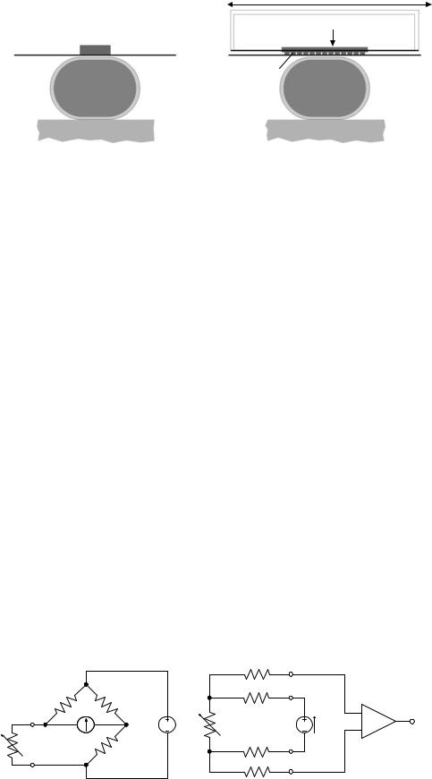
Figure 1. Applanation tonometry principle. (a) Single-element transducer. (b) Sensor array with pneumatic contact pressure control.
Pressure transducer
Artery
Bone
(a)
Applanation Tonometry. First conceived and implemented by Pressman and Newgard in the early 1960s, applanation tonometry (AT) measures the pulse pressure wave of a superficial artery with an externally applied transducer (6). The method requires the artery to be supported by an underlying rigid (i.e., bone) structure. Therefore, the method has been applied mainly to the temporal and the radial arteries; the last one being by far the most frequently employed measurement site. Figure 1a shows the general principle of the method. A pressure transducer is placed over the artery, and appropriate pressure is applied so as to partially flatten, or applanate, the artery. This ensures that the vessel wall does not exert any elastic forces perpendicular to the sensor face; therefore the sensor receives only internal arterial pressure changes caused by the arterial pulse. To obtain an accurate measurement it is crucial that the transducer is precisely centered over the artery, and that it is has stable support with respect to the surrounding tissue.
The original design used a single transducer that consisted of a rod of 2.5 mm2 cross-sectional area, which was pressed against the artery, and which transmitted arterial pressure to a strain gauge above it. This early design suffered from practical difficulties in establishing and maintaining adequate sensor position. In addition, Drzewiecki has shown that for accurate pressure readings, the transducer area needs to be small compared to artery diameter (ideally, < 1 mm wide), a requirement that early designs did not meet (1).
The development of miniaturized pressure sensor arrays in the late 1970s has alleviated these difficulties, leading to the development of commercial AT instruments by Colin Medical Instruments Corp., San Antonio, TX. These sensor arrays use piezoresistive elements, which essentially are membranes of doped silicon (Si) that show a change in electrical resistance when subjected to
|
Computer controlled translation |
Pressure chamber |
|
|
Contact pressure |
Skin |
Skin |
Multi-sensor |
|
array |
Artery |
Bone
(b)
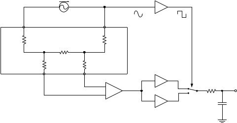
mechanical stress. Piezoresistivity is a quantum mechanical effect rooted in the dependence of charge carrier motility on mechanical changes in the crystal structure. Pressure-induced resistance changes in a monocrytalline semiconductor are substantially greater than in other available strain gauges. This sensitivity together with the possibility of using semiconductor fabrication techniques to create miniaturized structures makes piezoresistive elements ideal candidates for AT applications. The change in resistance is measured with a Wheatstone bridge (e.g., pictured in Fig. 2), which, together with suitable amplification, can be integrated on the same chip as the sensing element. While piezoresistance shows linear change with strain, the devices are strongly influenced by ambient temperature. Therefore, appropriate compensation measures have to be taken.
Figure 1b shows the schematic of a modern AT pressure sensor. Thirty-one piezoeresistive elements form the 4.1 10 mm large sensor array, which is created from a monolithic Si substrate. After placing the sensor roughly over the artery, the signal from each element is measured to determine whether the transducer is appropriately centered with respect to the vessel. If necessary, its lateral position is automatically adjusted with a micromotor drive. The sensor contact pressure is pneumatically adjusted to achieve appropriate artery applanation. To provide probe stability suitable for long-term studies, the device is strapped to the wrist together with a brace that immobilizes the hand in a slightly overextended position so as to achieve better artery exposure to the sensor field.
Because AT can accurately measure the pulse wave shape, not its absolute amplitude, the AT signal is calibrated with a separate oscillatory BP measurement on the ipsilateral arm. Calibration is performed automatically at predetermined intervals.
|
|
|
|
R pr1 |
|
|
(a) |
|
(b) |
|
|
|
A |
|
|
Rex1 |
|
Figure 2. (a) Wheatstone bridge |
R3 |
R1 |
R |
DC |
|
for sensitive detection of resistor |
B |
D DC |
Vout |
||
|
|
R ex2 |
|||
changes; gauge lead resistance dis- |
R |
R2 |
|
|
|
turbs measurement. (b) Four-wire |
|
|
R pr2 |
|
|
strain gauge measurement; influ- |
C |
|
|
|
|
|
|
|
|
||
ence of lead resistance is eliminated. |
|
|
|
|
|
|
|
|
|
|

In addition to fully automated long-term monitoring devices, simpler single-element transducers are offered for clinical and research applications (PulsePen by DiaTecne, Milan, Italy and SPT-301 by Millar Instruments, Inc., Houston, TX).
Plethysmography
Plethysmography (derived from the Greek words for ‘‘inflating’’ and ‘‘recording’’) is the general name of an investigative method that measures volume change of the body, or a part of it, in response to physiologic stimulation or activity. Specifically, it allows measuring dynamics of blood flow to/from the extremities for the diagnosis of peripheral vascular diseases.
Different approaches have been conceived to measure volume change of a limb, the earliest of which, reaching back to the end of the nineteenth century, were based on measuring the volume displacement in a water filled vessel in which the limb was sealed in (7,8). Even though accurate in principle, the method suffers from practical limitations associated with the need to create a satisfactory watertight seal; it has therefore largely been supplanted by other approaches. The most important methods currently used are strain gauge PG, impedance PG, and photo PG. The working principles and applications of each of these methods will be described in the following sections.
Strain Gauge Plethysmography. Introduced by Whitney in 1953 (9), strain gauge plethysmography (SPG) measures changes in limb circumference to deduce volume variations caused by blood flow activity. The strain gauge is a stretchable device whose electrical resistance depends on its length; for SPG, it is fitted under tension in a loop around the limb of interest. Pulsatile and venous blood volume changes induce stretching/relaxing of the gauge, which is translated into a measurable resistance variation. Measurement interpretation is based on the premise that the local circumference variation is representative of the overall change in limb volume.
Whitney introduced a strain gauge consisting of flexible tubing of length l made from silastic, a silicone-based elastomer, filled with mercury. Stretching of the tubing increases the length and decreases the cross-sectional area a of the mercury-filled space, leading to an increase in its resistance R according to
l2 |
|
R ¼ rm v |
(1) |
where rm denotes mercury’s resistivity (96 mV cm), and v is the mercury volume, v ¼ l a. Differentiation of Eq. 1. shows that the gauge’s change in resistance is proportional to its length variation (10):
DR |
¼ 2 |
Dl |
(2) |
R |
l |
Whitney’s original strain gauge design is still the most commonly used in SPG. Because of typical gauge dimensions and mercury’s resistivity, the devices have rather small resistance values, in the range of 0.5–5 V.
PERIPHERAL VASCULAR NONINVASIVE MEASUREMENTS |
237 |
The measured limb is often approximated as a cylinder of radius r, circumference C, length L, and volume V. By expressing the cylinder volume in terms of its circumference, V ¼ C2L/(4p), and then differentiating V with respect to C, it is shown that the fractional volume change is proportional to relative variations in circumference:
dV |
¼ 2 |
dC |
(3) |
|
|
|
|
||
V |
C |
|||
Because changes in C are measured by the strain gauge according to Eq. 1, the arm circumference is proportional to the tubing length, and so the following relationship holds:
DV |
¼ |
DR |
(4) |
|
|
||
V |
R |
Whitney used a Wheatstone bridge, a measurement circuit of inherently great sensitivity, to detect changes in gauge resistance. In this configuration, shown in Fig. 2a, three resistors of known value together with the strain gauge form a network, which is connected to a voltage source and a sensitive voltmeter in such a manner that zero voltage is detected when R1/R2 ¼ R3/R. In this case, the bridge is said to be balanced. Changes in strain, and therefore R, cause the circuit to become unbalanced, and a nonzero voltage develops between points B and D according to
VBD |
¼ |
R2 |
|
R |
(5) |
|
VAC |
R1 þ R2 |
R3 þ R |
|
|||
One disadvantage of the circuit is its nonlinear voltage response with respect to variations in R. For small changes, however, these nonlinearities remain small, and negligible errors are introduced by assuming a linear relationship.
A more significant shortcoming of the Wheatstone setup is that the measurement is influenced by the voltage drop across the lead resistance; especially for small values of R, such as those encountered in SPG applications, this can be a significant source of error. Therefore, modern SPG instruments use a so-called four-wire configuration, which excludes influences of lead resistance entirely. Figure 2b shows the concept. An electronic source is connected to the strain gauge with two excitation leads of resistance Rex1, Rex2, sending a constant current I through the strain gauge. Two probing leads with resistances Rpr1, Rpr2 connect the device to an instrumentation amplifier of high impedance Ramp Rpr1, Rpr2, which measures the voltage drop VSG ¼ I R across the strain gauge. Because VSG is independent of Rex1 and Rex2, and there is negligible voltage drop across Rpr1 and Rpr2, lead resistances do not influence the measurement of R.
Recently, a new type of plethysmography strain gauge has been introduced, which measures circumference variations in a special band that is worn around the limb of interest. The band, which has a flexible zigzag structure to allow longitudinal stretching, supports a nonstretching nylon loop, whose ends are connected to an electromechanical length transducer. Changes in circumference are thus translated into translational motion, which the transducer measures on an inductive basis, with 5 mm
238 PERIPHERAL VASCULAR NONINVASIVE MEASUREMENTS
accuracy (11). In evaluation studies, the new design performed comparable to traditional strain gauge designs (12).
Impedance Plethysmography. Electrical conductivity measurements on the human body for the evaluation of cardiac parameters were performed as early as the 1930s and 1940s. Nyboer is widely credited with the development of Impedance Plethysmography (IPG) for the measurement of blood flow to organs, and its introduction into clinical use (13–15).
The frequency-dependent, complex electrical impedance Z(f) of tissue is determined by the resistance of the interand intracellular spaces, as well as the capacitance across cell membranes and tissue boundaries. The IPG measurements are performed at a single frequency in the 50–100 kHz range, and only the impedance magnitude Z (not the phase information) is measured. Therefore, Z can be obtained by applying Ohms law
|
|
|
ˆ |
|
|
|
|
Z ¼ |
V |
|
(6) |
|
|
Iˆ |
|||
ˆ |
ˆ |
|
|
and current amplitude |
|
where V |
and I |
denote voltage |
|||
values, respectively.
In the mentioned frequency range, the resistivity of different tissues varies by about a factor of 100, from1.6 V m for blood to 170 V m for bone. Tissue can be considered a linear, approximately isotropic, piecewise electrically homogeneous volume conductor. Some organs, however, notably the brain, heart and skeletal muscles, show highly anisotropic conductivity (16).
Figure 3 shows a schematic for a typical four-electrode IPG setup. Two electrodes are used to inject a defined current into the body part under investigation, and two separate electrodes between the injection points measure the voltage drop that develops across the section of interest. The impedance magnitude Z is obtained, via Eq. 6, from the known current amplitude and the measured voltage amplitude. The four-electrode arrangement is used to eliminate the influence of the high skin impedance (Zs1 ¼ Zs4), which is 2–10 times greater than that of the underlying body
tissue (17). If the same two electrodes were used to inject the current as well as to pick up the voltage drop, the skin resistance would account for most of the signal and distort the information sought.
The current source generates a sinusoidal output in the described frequency range and maintains a constant amplitude of typically 1 mA. This provides sufficient signal noise ratio (SNR) to detect physiologic activity of interest but is 50 times below the pain threshold for the employed frequency range, and therefore well below potentially hazardous levels.
The voltage difference between the pick-up electrodes is measured with an instrumentation amplifier, whose input impedance is much greater than that of skin or underlying tissue. Therefore, the influence of skin impedance can be neglected, and the measurement yields the voltage drop caused by the tissue of interest. The output of the instrumentation amplifier is a sinusoidal voltage with amplitude proportional to the impedance of interest. The signal needs to be demodulated, that is, stripped of its carrier frequency, to determine the instantaneous amplitude value. This is done with a synchronous rectifier followed by a low pass filter, a technique also known as synchronous, lock-in, or homodyne detection. Figure 3 shows a possible analog circuit implementation; a discriminator, or zero-crossing detector, actuates a switch that, synchronously with the modulation frequency, alternately connects the buffered or inverted measured signal to a low pass filter. If phase delays over transmission lines can be neglected, this will generate a noninverted signal during one-half of a wave, say the positive half, and an inverted signal during the negative half wave. As a result, the carrier frequency is rectified. The low pass filter averages the signal to remove ripple and generates a signal proportional to the carrier frequency amplitude. Inspection shows that frequencies other than the carrier frequency (and its odd harmonics) will produce zero output.
Increasingly, the measured voltage is digitized by an analog-to-digital converter, and demodulation is achieved by a microprocessor through digital signal processing.
The measured impedance is composed of a large direct current (DC), component onto which a small (0.1–1%)
Figure 3. Four-lead tissue impedance measurement; the configuration mitigates influence of skin resistance (A1, instrumentation amplifier). Synchronous detection removes carrier signal.
ac current source |
|
Discriminator |
|
50...100 kHz, 1mA |
|||
|
|||
Zs1 |
Zs2 |
|
|
ZV |
Zs4 |
|
|
Zs3 |
|
||
|
|
1 |
|
|
+ |
Buffer |
|
|
|
||
|
− |
ZV |
|
|
A1 |
−1 |
|
Inverter

time-varying component is superimposed. The former is the constant impedance of the immobile tissue components, such as bone, fat, and muscle, and the latter represents impedance variations induced by volume changes in the fluid tissue components:most significantly, blood volume fluctuations in the vascular component. To obtain a quantitative relationship between measured impedance variations DZ and the change in blood volume, a simple electrical tissue equivalent may be considered, consisting of two separate, parallel-connected volume conductors of equal length L. One of these represents the immobile tissue components of impedance Z0. The other is assigned resistivity r and a variable cross-sectional area A, thereby modeling impedance changes caused by variations in its volume V according to the relationship
Zv ¼ r |
L |
¼ r |
L2 |
(7) |
|
A |
|
V |
|||
Here Zv denotes the variable compartment’s impedance, which is generally much greater than that of the immobile constituents. Therefore, the parallel impedance of both conductors can be approximated Z Z0 Zv. To obtain a functional relationship between the measured changes in impedance DZ and variations in blood volume DV, Eq. 7 is solved for V and differentiated with respect to Z. Making use of Z Z0 and dZ dZv yields
|
rL2 |
|
DV ¼ |
Z02 DZv |
(8) |
The IPG measurements do not allow independent determination of Z0 and Zv; however, the dc component of the IPG signal serves as a good approximation to Z0, while the ac part closely reflects changes in Zv. Low pass filtering of the IPG signal extracts the slowly varying dc components. Electronic subtraction of the dc part from the original signal leaves a residual that reflects physiologic impedance variations. The ac/dc separation can be implemented with analog circuitry. Alternatively, digital signal processing may be employed for this task. Digital methods help alleviate some of the shortcomings of analog circuits, especially the occurrence of slow signal drifts. In addition, softwarebased signal conditioning affords easy adjusting of processing characteristics, such as the frequency response, to specific applications.
Air Plethysmography. Air plethysmography (APG), also referred to as pneumoplethysmography, uses inflatable pressure cuffs with integrated pressure sensors to sense limb volume changes. The cuff is inflated to a preselected volume, at which it has snug fit, but at which interference with blood flow is minimal. Limb volume changes due to arterial pulsations, or in response to occlusion maneuvers with a separate cuff, cause changes in the measurement cuff internal pressure, which the transducer translates into electrical signals. The volume change is given by
DV ¼ V |
DP |
(9) |
P |
PERIPHERAL VASCULAR NONINVASIVE MEASUREMENTS |
239 |
The APG measurements can be calibrated with a bladder that is inserted between the limb and the cuff, which is filled with a defined amount of water. Because temperature changes influence air pressure inside the cuff, and it needs to be worn for a few minutes after inflation before starting the measurement, so the air volume can reach thermal equilibrium.
Photoplethysmography. Optical spectroscopic investigations of human tissue and blood reach back as far as the late nineteenth and early twentieth century, and Hertzman is widely credited with introducing photoplethysmography (PPG) in 1937 (18). The PPG estimates tissue volume changes based on variations in the light intensity transmitted or reflected by tissue.
Light transport in tissue is governed by two principle interaction processes; elastic scattering, that is, the random redirection of photons by the microscopic interfaces of the cellular and subcellular structures; second, photoelectric absorption by molecules. The scattering power of tissue is much greater (at least tenfold, depending on wavelength) than is the absorption, and the combination of both interactions cause strong dampening of the propagating light intensity, which decays exponentially with increasing distance from the illumination point. The greatest penetration depth is achieved for wavelengths in the 700–1000 nm range, where the combined absorption of hemoglobin (Hb) and other molecules show a broad minimum. Figure 4 shows the absorption spectra of Hb in its oxygenated (HbO2) and reduced, or deoxygenated, forms.
The PPG measurements in transmission are only feasible only for tissue thickness of up to a few centimeters. For thicker structures, the detectable light signal is too faint to produce a satisfactory SNR. Transmission mode measurements are typically performed on digits and the earlobes.
Whenever tissue is illuminated, a large fraction of the light is backscattered and exits the tissue in the vicinity of the illumination point. Backreflected photons that are detected at a distance from the light source are likely to have descended into the tissue and probed deeper lying structures (Fig. 5). As a general rule, the probing depth
] |
106 |
|
|
|
|
|
|
|
-1 |
|
|
|
|
|
|
|
|
M |
|
|
|
|
|
|
|
|
-1 |
105 |
|
|
|
|
|
|
|
coeff. [cm |
|
|
|
|
|
|
|
|
104 |
|
|
|
|
|
|
|
|
extinction |
|
|
Hb |
isosbestic point |
|
|||
|
|
|
|
|||||
|
|
|
|
|
||||
|
|
|
|
|
|
|
|
|
Molar |
103 |
HbO2 |
|
|
|
|
|
|
|
|
|
|
|
|
|||
|
|
|
|
|
|
|
||
|
102 |
|
|
|
|
|
|
|
|
400 |
500 |
600 |
700 |
|
800 |
900 |
1000 |
|
|
|
Wavelength [nm] |
|
|
|||
Figure 4. Hemoglobin |
spectra; |
typical |
PPG |
wavelength for |
||||
oxygen saturation measurement are 660 and 940 nm.
240 PERIPHERAL VASCULAR NONINVASIVE MEASUREMENTS
Source |
Detector |
Epidermis
Capillaries
Superficial
plexus
Dermis
Figure 5. Schematic of the probed Deep plexus tissue volume in PPG reflection
geometry.
equals about half the source-detector separation distance. The separation represents a tradeoff between probing volume and SNR; typical values are on the order of a few millimeters to a few centimeters. Reflection-geometry PPG can be applied to any site of the body.
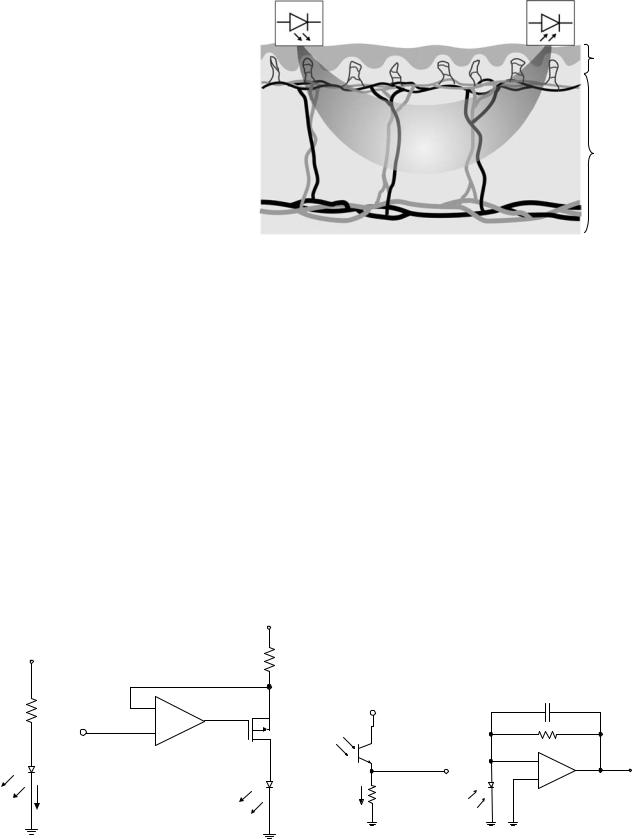
Originally, incandescent light sources were used for PPG. These have been replaced with light emitting diodes (LED), owing to the latter devices’ superior lifetime, more efficient operation (less heat produced), and desirable spectral properties. The LED technology has vastly evolved over the last 20 years, with a wide range of wavelengths— from the near-infrared (NIR) to the ultraviolet (UV) —and optical power of up to a tens of milliwatts currently available. These devices have a fairly narrow emission bandwidth, 20–30 nm, which allows spectroscopic evaluation of the tissue. The light-emitting diode (LEDs) are operated in forward biased mode, and the produced light intensity is proportional to the conducted current, which typically is on the order of tens of milliamps. Because in this configuration, the device essentially presents a short circuit to any voltage greater than its forward drop VLED (typically 1– 2 V), some form of current control or limiting circuitry is
|
|
+Vcc |
(a) |
(b) |
|
+Vcc |
|
R |
|
|
|
Rlim |
− |
|
|
Vin |
|
|
+ |
Q1 |
LED |
A1 |
|
|
|
|
|
|
LED |
ILED |
|
|
Figure 6. LED drive circuits. (a) Simple current limiting resistor.
(b) Voltage controlled current source.
required. In the simplest case, this is a current-limiting resistor Rlim in series with the diode (Fig. 6a). The value of
Rlim is chosen so that ILED ¼ (Vcc VLED)/Rlim is sufficient to drive the LED, typically on the order of tens of milli-
amps, but does not exceed the maximum permissible value. Depending on the voltage source, this results in adequate output stability. Often, there is a requirement to modulate or adjust the diode output intensity. In this case, an active current source is better suited to drive the LED. Figure 6b shows the example of a voltage-controlled current source with a boost field effect transistor. Here, the light output is linearly dependent on the input voltage from zero to maximum current; the latter is determined by LEDs thermal damage threshold.
Either phototransistors (PT) or photodiodes (PD) are used as light sensors for PPG. Both are semiconductor devices with an optically exposed pn junction. Photons are absorbed in the semiconductor material, where they create free charges through internal photoelectric effect. The charges are separated by the junction potential, giving rise to a photocurrent Ip proportional to the illumination intensity. While a PD has no internal gain mechanism and requires external circuitry to create a suitable signal, the PT (like any transistor) achieves internal current amplification hFE, typically by a factor of 100. Figure 7a shows how a load resistor is used to convert the PT output current to voltage that is approximately proportional to
(a) |
|
(b) |
Vcc |
|
|
|
|
Cf |
C |
|
Rf |
|
|
|
E |
|
− |
Vout |
PD |
Vout |
+ |
||
ICE RL |
|
A1 |
Figure 7. Light detection circuits. (a) Phototransistor operation (VCE ¼ collector-emitter voltage). (b) Use of photodiode with current-to-voltage converter (transimpedance amplifier).

the incident light according to
VL ¼ ICERL ¼ hFEIpRL |
(10) |
hFE unavoidably depends on a number of factors including Ip and VCE, thus introducing a nonlinear circuit response. In addition, the PT response tends to be temperature sensitive. The light sensitivity of a PT is limited by its dark current, that is, the output at zero illumination, and the associated noise. The largest measurable amount of light is determined by PT saturation, that is, when VL approaches Vcc. The device’s dynamic range, that is, the ratio between the largest and the smallest detectable signal is on the order of three-to-four orders of magnitude.
Figure 7b shows the use of a PD with photoamplifier. The operational amplifier is configured as a current-to- voltage converter and produces an output voltage
Vo ¼ IpRf |
(11) |
Capacitor Cf is required to reduce circuit instabilities. Even though compared to (a) this circuit is more costly and bulky because of the greater number of components involved, it has considerable advantages in terms of temperature stability, dynamic range, and linearity. The PD current varies linearly with illumination intensity over seven-to-nine orders of magnitude. The circuit’s dynamic range is determined by the amplifier’s electronic noise and its saturation, respectively, and is on the order of four decades. Proper choice of R determines the circuit’s working range; values in the 10–100 MV range are not uncommon.
It is clear from considering the strong light scattering in tissue that the PPG signal contains volume-integrated information. Many models of light propagation in tissue based on photon transport theory have been developed that are capable of computing realistic light distributions even in inhomogeneous tissues, such as the finger (19). However, it is, difficult, if not impossible, to exactly identify the sampled PPG volume because this depends critically on the encountered optical properties as well as the boundary conditions given by the exact probe placement, digit size and geometry, and so. These factors vary between individuals, and even on the same subject are difficult to quantify or even to reproduce. Therefore, PPG methods do generally not employ a model-based approach, and the origin of the PPG signal as well as its physiologic interpretation has been an area of active research (20–23).
The PPG signals are analyzed based on their temporal signatures, and how those relate to known physiology and empirical observations. The detected light intensity has a static, or dc component, as well as a time-varying ac part. The former is the consequence of light interacting with static tissues, such as skin, bone, and muscle, while the latter is caused by vascular activity. Different signal components allow extraction of specific anatomical and physiological information. For example, the signal component showing cardiac pulsation, also called the digital volume pulse (DVP), can be assumed to primarily originate in the arterial bed, a premise on which pulse oximetry, by far the most widely used PPG application, is based. This method obtains two PPG signals simultaneously at two wave-
PERIPHERAL VASCULAR NONINVASIVE MEASUREMENTS |
241 |
lengths that are spectrally located on either side of the isosbestic point. The ratio of the DVP peak amplitudes for each wavelength, normalized by their respective dc components, allows assessment of quantitative arterial oxygen saturation.
A number of other applications of the DVP signal have been proposed or are under investigation. For example, the DVP waveform is known to be related to the arterial blood pressure (ABP) pulse. Using empirically determined transfer functions, it is possible to derive the ABP pulse from PPG measurements (24).
Another potential use of arterial PPG is the assessment of arterial occlusive disease (AOD). It is known that the arterial pulse form carries information about mechanical properties of the peripheral arteries, and PPG has been investigated as a means to noninvasively assess arterial stiffness. To better discriminate features in the PPG signal shape, the second derivative of the signal is analyzed (second-derivative plethysmography, SDPTG) (23).
The PPG is furthermore used for noninvasive peripheral BP monitoring in the vascular unloading technique.
Continuous Wave Doppler Ultrasound
Doppler ultrasound (US) methods are capable of measuring blood flow velocity and direction by detecting the Doppler shift in the ultrasound frequency that is reflected by the moving red blood cells. The acoustic Doppler effect is the change in frequency of a sound wave that an observer perceives who is in relative motion with respect to the sound source. The amount of shift Df in the US Doppler signal is given by (25)
D f ¼ |
2 f0vbcosQ |
(12) |
c |
where f0 is the US frequency, vb is the red blood cell velocity, Q is the angle between the directions of US wave propagation and blood flow, and c is the speed of sound in tissue. Equation 12 demonstrates a linear relationship between blood flow and US Doppler shift. It is also seen that the shift vanishes if the transducer is perpendicular to the vessel because there is no blood velocity component in the direction of wave propagation. The algebraic sign of the shift depends on the flow direction (toward/away from) with respect to the transducer and is hence influenced by angle Q. A factor of two appears in Eq. 12 because the Doppler effect takes place twice; the first occurs when the red blood cell perceives a shift in the incoming US wave, and the second shift taks place when this frequency is backreflected toward the transducer. Using typical values for the quantities in Eq. 12 (f0 ¼ 5 MHz, vb ¼ 50 cm s 1, Q ¼ 458) yield frequency shifts of 2.3 kHz, which falls within the audible range (25).
Because the shift is added to the US frequency, electronic signal processing is used to remove the high frequency carrier wave. Analog demodulation has been used for this purpose; by mixing, that is, multiplying, the measured frequency with the original US frequency and low pass filtering the result, the carrier wave is removed, and audiorange shift frequencies are extracted. In so-called quadrature detection, this demodulation process yields two

242 PERIPHERAL VASCULAR NONINVASIVE MEASUREMENTS
separate signals, one for flow components toward the detector, and one for flow away from it. Modern instruments typically employ digital signal processing, such as fast Fourier transformation (FFT), to accomplish this.
Continuous wave (CW) Doppler refers to the fact that the measurement is performed with a constant, nonmodulated US wave (i.e., infinite sine-wave). This technology does not create echo pulses, and hence does not allow any form of depth-profiling or imaging. Its advantages are its simplified technology, and that it is not restricted to a limited depth or blood velocity. Because the signal is generated continuously, CW transducers require two separate crystals, one for sound generation, and one for detection. The two elements are separated by a small distance and are inclined toward each other. The distance and angle between the elements determine the overlap of their respective characteristics, and thus determine the sensitive volume. All blood flow velocity components within this volume contribute to the Doppler signal.
In the simplest case, the measured frequency shift is made audible through amplification and a loudspeaker, and the operator judges blood velocity from the pitch of the tone (higher pitch ¼ faster blood movement). These devices are used in cuff-based arterial pressure measurements, to detect the onset of pulsation. They also permit qualitative assessment of arterial stenosis and venous thrombosis. More sophisticated instruments display the changing frequency content of the signal as a waveform (velocity spectral display). Doppler spectra are a powerful tool for the assessment of local blood flow in the major vessels, especially when combined with anatomical US images (Duplex imaging, see section on imaging methods).
Peripheral Vascular Measurements
The following is a description of peripheral vascular measures that can be derived with the nonimaging techniques described in the preceding sections.
Assessment Of Peripheral Arterial Occlusive Disease.
Peripheral arterial occlusive disease (PAOD) is among the most common peripheral arterial diseases (26), with a reported prevalence as high as 29% (27). The PAOD is usually caused by atherosclerosis, which is characterized by plaque buildup on the inner-vessel wall, leading to congestion, and hence increased blood flow resistance. Risk factors for PAOD are highly correlated with those for coronary artery disease, and include hypertension, smoking, diabetes, hyperlipidemia, age, and male sex (27–29). A symptom of PAOD is intermittent claudication, that is, the experience of fatigue, pain, and cramping of the legs during exertion, which subsides after rest. Ischemic pain at rest, gangrene, and ulceration frequently occur in advanced stages of the disease (29,30).
Ankle Brachial Index Test. The Ankle Brachial Index (ABI) is a simple and reliable indicator of PAOD (31), with a detection sensitivity of 90% and specificity of 98% for stenoses of >50% in a major leg artery (27,29). The ABI for each leg is obtained by dividing the higher of the posterior and anterior tibial artery systolic pressures for
Table 1. Ankle-Brachial Index (ABI) staging after ()
AB Ratio Range |
Stage |
|
|
1.0–1.1 |
Normal |
< 1.0 |
Abnormal, possibly asymptomatic |
0.5–0.9 |
Claudication |
0.3–0.5 |
Claudication, rest pain, severe |
|
occlusive disease |
< 0.2 |
Ischemia, gangrenes |
|
|
that leg by the greater of the leftand right-brachial artery systolic pressures. In normal individuals both systolic values should be nearly equal, and ABIs of 1.0–1.1 are considered normal. In PAOD, the increased peripheral arterial resistance of the occluded vessels causes a drop in blood pressure, thus diminishing the ABI. Because of measurement uncertainties, ABI values of < 0.9 generally are considered indicative of PAOD (27,29). Table 1 shows a scheme for staging of disease severity according to ABI values, as recommended by the Society of Interventional Radiology (SIR) (32).
The ABI test is performed with the patient in a supine position, and inflatable pressure cuffs are used to occlude the extremities in the aforementioned locations. The systolic pressure is determined by deflating the cuff and noting the pressure at which pulse sounds reappear. The audio signal from a CW Doppler instrument is used to determine the onset of arterial pulse sounds. Although the test can be performed manually with a sphygmomanometer, there are dedicated vascular lab instruments that automatically control the pressure cuff, register the pressure values, and calculate the ABI. Such instruments are commercially available, for example, from BioMedix,MN, Hokanson, WA, and Parks Medical Electronics, OR.
The primary limitation of the ABI test is that arterial calcifications, such as are common in diabetics, can resist cuff pressure thus causing elevated pressure readings. In those patients, the toe pressure as determined by PPG or SPG may be used because the smaller digital arteries do not develop calcifications (29). The normal toe systolic pressure (TSP) ranges from 90 mmHg to 100 mmHg, or 80% to 90% brachial pressure. The TSP < 30 mmHg (3.99 kPa) is indicative of critical ischemia (33). Also, pulse volume recordings (PVR, see below) are not affected by calcifications (26).
Segmental Systolic Pressure. Segmental Systolic Pressure (SSP) testing is an extension of the ABI method, wherein the arterial systolic pressure is measured at multiple points on the leg, and the respective ratios are formed with the higher of the brachial systolic readings. As is the case for ABI testing, a low ratio for a leg segment indicates occlusion proximal to the segment. By comparing pressures in adjacent segments, and with the contralateral side, SSP measurements offer a way to locate pressure drops and thus roughly localize occlusions. Typically, three to four cuffs are placed on each leg; one or two on the thigh, one below the knee, and one at the ankle.
The SSP technique suffers from the same limitation as does the ABI test, that is, it produces falsely elevated readings for calcified arteries. Again, TSP and PVR are
advised for patients where calcifications might be expected because of known predisposition (e.g., diabetics), or unusual high ABI (> 1.5) (26).
Pulse Volume Recording/Pulse Wave Analysis. Pulse volume recording (PVR), a plethysmographic measurement, is usually combined with the ABI or SSP test. Either the pressure cuffs used in these measurements are equipped with a pressure sensor so they are suitable for recordind volume changes due to arterial pulsation, or additional strain gauge sensors are used to obtain segmental volume pulsation. In addition to the leg positions, sensors may be located on the feet, and PPG sensors may be applied to toes. Multiple waveforms are recorded to obtain a representative measurement; for example, the Society for Vascular Ultrasound (SVU) recommends a minimum of three pulse recordings (34). The recorded pulse amplitudes reflect the local arterial pressure, and the mean amplitude, obtained by integrating the pulse, is a measure of the pulse volume. The pulsatility index, the ratio of pulse amplitude over mean pulse volume serves as an index for PAOD, with low values indicating disease (26).
Besides its amplitude and area, the pulse contour can be evaluated for indications of PAOD in a method referred to as pulse wave analysis (PWA). The normal pulse has a steep (anacrotic) rise toward the systolic peak, and a slower downward slope, representing the flow following the end of the heart’s left ventricular contraction. The falling slope is interrupted by a short valley (the dicrotic notch), which is caused by the closing of the aortic valve. The details of the pulse shape are the result of the superposition of the incoming arterial pulse and backward-traveling reflections from arterial branchings and from the resistance caused by the small arterioles, as well as from atherosclerotic vessels (35). The pulse shape distal to occlusions tends to be damped and more rounded, and loses the dicrotic wave. Combined SSP and PVR recording has been reported over 90% accurate for predicting the level and extent of PAD (26).
Recently, PWA has increasingly been used to infer central, that is, aortic, arterial parameters from peripheral arterial measures, typically obtained from tonometric measures on the radial artery. These methods, which are commercialized for example by Atcor Medical, Australia and Hypertension Diagnostics, Inc, MN, rely on analytic modeling of transfer functions that describe the shaping of the pulse from the aorta to the periphery. These analytical functions are typically based on models mimicking the mechanical properties of the arterial tree by equivalent circuits (so-called Windkessel models) representing vascular resistances, capacitances, and inductances (36–38). From the derived aortic waveform, parameters are extracted that indicate pathologic states, such as hypertension and central arterial stiffness. One example is the augmentation index, the pressure difference in the first and second systolic peak in the aorta (39,40).
Pulse wave velocity (PWV) depends on arterial stiffness, which is known to correlate with increased cardiovascular risks. The PWV is established by measuring pulse waves on more than one site simultaneously, and dividing their respective separation difference from the heart by the time difference between the arrivals of comparable wave form
PERIPHERAL VASCULAR NONINVASIVE MEASUREMENTS |
243 |
features. Peripheral PWV measurements on toes and fingers have been conducted with PPG (41).
It was recently shown that arterial stiffness assessed from PWA and PVA on multisite peripheral tonometric recording correlates with endothelial function. The latter was assessed by US measurements of brachial arterial diameter changes in response to a reactive hyperemia maneuver (42). There is increasing clinical evidence that PWA can serve as a diagnostic tool for hypertension and as a cardiac disease predictor (43).
CW Doppler Assessment. Velocity spectral waveform CW Doppler is useful for assessing peripheral arterial stenoses. The Doppler waveform obtained from a normal artery shows a triphasic shape; there is a strong systolic peak, followed by a short period of low amplitude reversed flow, reversing again to a small anterograde value during mid-diastole. Measuring at a stenosis location shows a waveform of increased velocity and bior monophasic behavior. Measurements distal to stenosis appear monophasic and dampened (26,33).
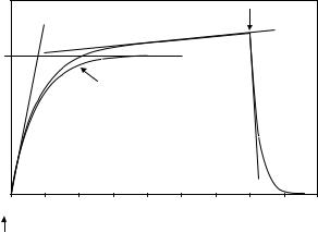
Venous Congestion Plethysmography. The described PG methods are most valuable for the assessment of peripheral vascular blood flow parameters for the diagnosis of peripheral vascular diseases (PVD). Venous congestion PG (VCP), also called venous occlusion PG (VOP), allows the measurement of a variety of important vascular parameters including arterial blood flow (Qa), venous outflow (Qvo), venous pressure (Pv), venous capacitance (Cv), venous compliance (C), and microvascular filtration. In VCP, a pressure cuff is rapidly inflated on the limb under investigation to a pressure, typically between 10 (1.33 kPa) and 50 mmHg (6.66 kPa), sufficient to cause venous occlusion, but below the diastolic pressure so that arterial flow is not affected. Blocking the venous return in this fashion causes blood pooling in the tissue distal to the cuff, an effect that can be quantified by measuring volume swelling over time with PG. Figure 8 sketches a typical
|
1 |
|
|
|
|
|
Cuff release |
||
|
|
|
|
|
|
|
3 |
|
|
|
|
|
|
|
|
|
|
|
|
Cv |
|
|
|
|
|
|
|
|
|
(a.u.) |
|
|
4 |
|
|
|
|
|
|
Volume change |
|
|
|
|
|
|
|
|
|
|
|
|
|
|
|
|
|
|
|
|
|
|
|
|
|
|
2 |
|
|
0 |
20 |
40 |
60 |
80 |
100 |
120 |
140 |
160 |
180 |
Cuff inflation |
|
Time (s) |
|
|
|
|
|||
Figure 8. Schematic of typical VCP response curve. (1), asymptotic arterial blood flow; (2), asymptotic venous outflow; (3), swelling due to filtration; (4), effect of venous blood pooling only, obtained by subtracting the filtration component (3); Cv, venous capacitance.
244 PERIPHERAL VASCULAR NONINVASIVE MEASUREMENTS
volume response curve. Upon cuff inflation, an exponential increase in volume is observed, which is caused by the filling of postcapillary compliance vessels, and for which the time constant is 15 s in healthy individuals (44). The initial rate of swelling (indicated by asymptote 1), expressed in (mL min 1), is a measure of the arterial blood flow. When the venous pressure reaches the cuff pressure, blood can again flow out, and the relative volume increase reaches a plateau, which equals Cv. If Cv is measured for different occlusion pressure values, the slope of the Cv versus pressure curve yields C (in mL mmHg 1 10 2). Upon cuff release, the VCP curve shows fast exponential decay (on the orders of seconds), whose initial rate (indicated by asymptote 2) is a measure for Qvo (45,46). With rising venous pressure an increase in fluid leakage, or filtration, takes place from the veins into the interstitial space, leading to additional tissue volume increase. Therefore, the PG response shows a second slow exponential component with a time constant on the order of 800 s (asymptote 3), from which can be deduced the capillary filtration capacity CFC (11).
Another application of VCP is the noninvasive diagnosis of deep vein thrombosis (DVT). The presence of venous blood clots impacts on venous capacitance and outflow characteristics. It has been shown that the combined measurement of Cv and Qvo may serve as a diagnostic discriminator for the presence of DVT (45). A computerized SPG instrument is available (Venometer, Amtec Medical Ltd, Antrim, Northern Ireland), which performs a fully automated VCP measurement and data analysis for the detection of DVT (47).
Laser Doppler Flowmetry
Laser Doppler flowmetry (LDF) is a relatively young method of assessing the perfusion of the superficial microvasculature. It is based on the fact that when light enters tissue it is scattered by the moving red blood cells (RBC) in the superficial vessels (see PPG illustration in Fig. 5), and as a result the backscattered light experiences a frequency (Doppler) shift. For an individual scattering event, the shift magnitude can be described exactly; it depends on the photon scattering angle and the RBCs velocity, and it is furthermore related to the angular orientation of blood flow with respect the path directions of the photon before and after the scattering event. In actual tissue measurements, it is impossible to discern individual scattering events, and the obtained signals reflect stochastic distributions of scattering angles and RBC flow directions and velocities present in the interrogated volume.
In its simplest form, an LDF measurement is obtained by punctual illumination of the tissue of interest with a laser source, and by detecting the light that is backscattered at (or close to) the illumination site with a photodetector, typically a photodiode. The laser is a highly coherent light source, that is, its radiation has a very narrow spectral bandwidth. The spectrum of the backscattered light is broadened because it contains light at Doppler frequencies corresponding to all scattering angles and RBC motions occurring in the illuminated volume. Because of typical flow speeds encountered in vessels, the maximum
Doppler shifts encountered are on the order of 20 kHz, which corresponds to a relative frequency variation of10 10. Frequency changes this small can be detected because the shifted light components interfere with the unscattered portion of the light, causing a ‘‘beat signal’’ at the Doppler frequency. This frequency, which falls roughly in the audio range, is extracted from the photodetector signal and further processed. The small amount of frequency shift induced by cell motion is the reason that spectrally narrow, high quality laser sources (e.g., HeNe gas lasers or single-mode laser diodes) are required for LDF measurements.
The basic restriction of LDF is its limited penetration depth. The method relies on interference, an effect that requires photon coherence. Multiple scattering, however, such as experienced by photons in biological tissues, strongly disturbs coherence. For typical tissues, coherence is lost after a few millimeters of tissue. The sensitive volume of single-point LDF measurements is therefore on the order of 1 mm3.
Single-point LDF measurements are usually performed with a fiberoptic probe, which consist of one transmitting fiber and one adjacent receiving fiber. Typical distances between these are from a few tenths of a millimeter to > 2 mm. According to light propagation theory (see section on PPG), farther separations result in deeper probing depths, however, because of coherence loss, the SNR decreases exponentially with increasing distance, limiting the maximum usable separation.
The use of a probe makes a contact-based single-point measurement very convenient. Fiber-based probe have been developed that implement several receivers at different distances from the source (48). This allows a degree of depth discrimination of the measured signals, within the aforementioned limits.
The LDF signal is analyzed by calculation the frequency power spectrum of the measured detector signal, usually after band-pass filtering to exclude low frequency artifacts and high frequency noise. From this the so-called flux or perfusion value—a quantity proportional to the number of RBCs and their root-mean-squared velocity, stated in arbitrary units—is obtained. It has been shown that the flux is proportional to the width the measured Doppler power spectrum, normalized to optical power fluctuations in the setup (49).
Laser Doppler imaging (LDI) is an extension of the LDF technique that allows the instantaneous interrogation of extended tissue areas up to tens of centimeters on each side. Two approaches exist. In one implementation, the laser beam is scanned across the desired field of view, and a photodetector registers the signal that is backreflected at each scanning step. In another technology, the field of view is broadly illuminated with one expanded laser beam, and a fast CMOS camera is used to measure the intensity fluctuations in each pixel, thus creating an image. This second approach, while currently in a stage of relative infancy, shows the potential for faster frame rates than the scanning imagers, and it has the advantage of avoiding mechanical components, such as optical scanners (50).
The LDF/LDI applications include the assessment of burn wounds, skin flaps, and peripheral vascular perfusion
problems, such as in Raynaud’s disease or diabetes. The vascular response to heating (51) and the evaluation of carpal tunnel syndrome also have been studied (52).
IMAGING METHODS
This section provides an overview of existing medical imaging methods, and how they relate to vascular assessment. Included here are imaging modalities that involve the use of contrast agents or of radioactive markers, even though these methods are not considered noninvasive in the strictest sense of the word.
Ultrasound Imaging
Structural US imaging, especially when combined with Doppler US methods, is at present the most important imaging technique employed in the detection of PVD.
Improvements in ultrasound imaging technology and data analysis methods have brought about a state in which ultrasonic images can, in some circumstances, provide a level of anatomical detail comparable to that obtained in structural X-ray CT images or MRIs (53,54). At the same time, dynamic ultrasound imaging modalities can readily produce images of dynamic properties of macroscopic blood vessels (55,56). The physical phenomenon underlying all the blood-flow-sensitive types of ultrasound imaging is the Doppler effect, wherein the frequency of detected ultrasonic energy is different from that of the source, owing to the interactions of the energy with moving fluid and blood cells as it propagates through tissue. Several different varieties have become clinically important.
The earliest, most basic version of dynamic ultrasound imaging is referred to as color flow imaging (CFI) or color Doppler flow imaging (CDFI). Here, the false color value assigned to each image pixel is a function of the average frequency shift in that pixel, and the resulting image usually is superimposed upon a coregistered anatomic image to facilitate its interpretation. Interpretation of a CDFI image is complicated by, among other factors, the dependence of the frequency shift on the angle between the transducer and the blood vessels in its field of view. In addition, signal/noise level considerations make it difficult to measure low but clinically interesting flow rates. Many of these drawbacks were significantly ameliorated by a subsequently developed imaging modality known as either power flow imaging (PFI) or power Doppler imaging (PDI) (57). The key distinction between PDI and CDFI is that the former uses only the amplitude, or power, of ultrasonic energy reflected from erythrocytes as its image-forming information; in consequence, the entire contents of a vessel lumen have a nearly uniform appearance in the resulting displayed image (58).
The greatest value of Doppler imaging lies in the detection and assessment of stenoses of the larger arteries, as well as in the detection of DVT.
An increasingly employed approach to enhancing ultrasound images, at the cost of making the technique minimally invasive, is by introducing a contrast agent. The relevant contrast agents are microbubbles, which are microscopic, hollow, gas-filled polymer shells that remain
PERIPHERAL VASCULAR NONINVASIVE MEASUREMENTS |
245 |
confined in the vascular space and strongly scatter ultrasonic energy (59). It has been found that use of microbubbles permits a novel type of Doppler-shift-based ultrasound imaging, called contrast harmonic imaging (CHI). The incident ultrasound can, under the correct conditions, itself induce oscillatory motions by the microbubbles, which then return reflections to the transducer at not only the original ultrasonic frequency, but also at its second and higher harmonics. While these signals are not high in amplitude, bandpass filtering produces a high SNR, with the passed signal basically originating exclusively from the vascular compartment of tissue (60). The resulting images can have substantially lower levels of ‘‘clutter’’ arising from nonvascular tissue, in comparison to standard CDFI or PDI methods.
Magnetic Resonance Imaging
Magnetic resonance imaging (MRI) is certainly the most versatile of the imaging modalities, and give the user the ability to study and quantify the vasculature at different levels. That is, depending on the details of the measurement, the resulting image may principally confer information about bulk blood flow (i.e., rates and volumes of blood transport in macroscopic arteries and veins), or about perfusion (i.e., amount of blood delivered to capillary beds within a defined time interval). The methods commonly employed to perform each of these functions are given the names magnetic resonance angiography (MRA) and perfusion MRI, respectively. As is the case for the other types of imaging treated here, each can be performed either with or without administration of exogenous contrast agents, that is, in either a noninvasive or a minimally invasive manner (61,62).
Magnetic Resonance Angiography. The MRA methods fall into two broad categories. The basic physical principle for one is flow-related enhancement (FRE), in which the pulse sequence employed has the effect of saturating the spins of 1H nuclei in the nonmoving portion of the selected slice (63,64). Blood flow that has a large component of motion perpendicular to that slice remains significantly less saturated. Consequently, more intense MR signals arise from the blood than from the stationary tissues, and the contents of blood vessels are enhanced in the resulting image. Subtraction of a static image obtained near the start of the data collection sequence permits even greater enhancement of the blood vessel contents. A drawback of this approach is that vessels that lie within the selected slice, with the direction of blood flow basically parallel to it, do not experience the same enhancement.
A phase contrast mechanism is the basic physical principle for the second category of MRA techniques (65,66). Position-selective phase shifts are induced in 1H nuclei of the selected slice via the sequential imposition of at least two transverse gradients that sum to a constant value across the slice. The effect is to induce zero net phase shifts among nuclei that were stationary during the gradient sequence, but a nonzero, velocity-dependent net phase shift on those that were in motion. The net phase shifts associated with the flowing blood are revealed in the
246 PERIPHERAL VASCULAR NONINVASIVE MEASUREMENTS
resulting image, again, especially following subtraction of an image derived from data collected before the phase contrast procedure.
Perfusion MRI. Early developments in this field necessarily involved injection of a MR contrast agent that has the effect of inducing a sharp transient drop in signal detected as the contrast bolus passes through the selected slice (67). As with many dynamic MRI techniques, the bulk of the published work is geared toward studies of the brain, where, provided that the blood–brain barrier is intact, the method’s implicit assumption that the contrast agent remains exclusively within the vascular space usually is justified. A sufficiently rapid pulse sequence allows the operator to generate curves of signal intensity vs. time, and from these one can deduce physiological parameters of interest, such as the cerebral blood flow (CBF), cerebral blood volume (CBV), and mean transit time (MTT) (67,68).
The minimally invasive approach described in the preceding paragraph remains the most common clinically applied type of perfusion MRI. A noninvasive alternative would have advantages in terms of permissible frequency of use, and would be of particular value in situations where pathology or injury has disrupted the blood–brain barrier. It also would make it possible to obtain perfusion images of other parts of the body than just the brain. Such an alternative exists, in the form of a set of methods known collectively as arterial spin labeling (ASL) (67) or arterial spin tagging (69). The common feature of all these techniques is that the water component of the blood is itself used as a contrast agent, by applying a field gradient that inverts the spins of 1H nuclei of arterial blood before they enter the slice selected for imaging. The signal change induced by this process is smaller than that resulting from injection of a contrast agent, however, so that requirements for high SNRs are more exacting, and subtraction of a control image a more necessary step.
An increasingly popular and important functional MRI technique is blood-oxygen-level-dependent (BOLD) imaging (67,70). This type of imaging produces spatial maps determined by temporal fluctuations in the concentration of deoxygenated hemoglobin, which serves as an endogenous, intravascular, paramagnetic contrast agent. The physiological importance of BOLD images is that they reveal spatial patterns of tissue metabolism, and especially of neuronal activity of the brain. However, careful examination of the BOLD signal indicates that it depends, in a complex way, on many vascular and non-vascular tissue parameters (67,71). As such, it is not (yet) a readily interpretable method for specifically studying peripheral vasculature.
Fast X Ray Computed Tomography
As data acquisition speeds, and consequently repetition rates, for X ray computed tomography (CT) imaging have increased over the last couple of decades, previously unthinkable dynamic imaging applications have become a reality. The most direct approach taken along these lines is to rapidly acquire sequences of images of a slice or
volume of interest and then examine and interpret, at any desired level of mathematical sophistication, temporal variations in the appearance of tissue structures in the images. Of course this approach is well suited to studying only organs whose functionality entails changes in shape or volume, such as the heart and lungs, and these have been the subject of many fast CT studies.
The functioning of many other organs, such as the kidneys (72), is related to the flow of blood and/or locally formed fluids, but does not involve gross changes in size or shape. In these cases it is necessary to introduce one or more boluses of X ray contrast agents, and to use fast CT to monitor their transit (73). While these methods violate the strict definition of noninvasive procedure, we include them in this synopsis out of consideration of the fact that the health risks associated with the contrast agents ordinarily are minor in relation to those imposed by the ionizing radiation that forms the CT images. For quantitation of regional blood flow and other dynamic vascular parameters, these techniques invariably employ some version of indicator dilution theory (73).
Indicator Dilution Approach
In one clinically important example, it has been found that the detected X ray CT signal changes in a quantifiable manner following inhalation of a gas mixture containing appreciable levels of nonradioactive isotopes of xenon (typically 33% Xe and 67% O2, or 30% Xe, 60% O2, 10% air) (75– 77). A variety of techniques based on this phenomenon, and referred to as stable xenon-enhanced CT or sXe–CT, were subsequently developed. The common feature is inhalation of a Xe-enriched gas mixture followed by repetitive scanning to monitor the wash-in and/or wash-out of the Xeaffected signal (75). However, while negative side effects are uncommon, they are known to occur (77). Consequently, the sXe/CT technique is applied almost exclusively to cerebral vascular imaging studies, in cases where there is a diagnosed injury or pathology (75).
Qualitatively similar approaches, known collectively as perfusion CT, that are based on monitoring the time course of passage of an injected bolus of an iodinated contrast agent, also have been developed (74,78,79). Of course, these are even more invasive than the approaches based on inhalation an inert gas. Conflicting assertions (80) have been made regarding which of two approaches, injection or inhalation based, give superior results.
Positron Emission Tomography with 15O
Strictly speaking, all forms of positron emission tomography (PET) imaging (as do all other nuclear medicine procedures) violate the formal definition of noninvasive measurements. The 2.1 min half-life of the isotope 15O, which is brief relative to those of the other commonly used positron emitters, makes 15O-labeled water a useful indicator of blood flow in dynamic PET measurements (81,82). Of course, as a practical matter radioisotope imaging methods cannot be used on a large scale for research or for clinical screening purposes. Medical literature on 15O- PET-based vascular studies, understandably, also focuses
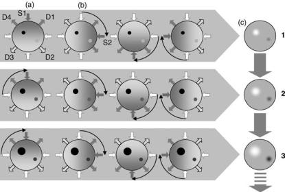
almost exclusively on studies of circulation in the brain, in subjects with diagnosed vascular pathologies such as arteriovenous malformations (81).
Temporal-Spectral Imaging
A new area of investigation and technology development involving assessment of blood delivery to the periphery includes the use of optical array measurements combined with image formation and analysis capabilities. The basic concept, referred to as temporal-spectral imaging (TSI) (83), considers the functional interactions between peripheral tissues and their blood supply, and the added information that is attainable from a time series of volumetric images of tissue, where the latter are reconstructed from optical measurements of the hemoglobin signal. The information content of the measurement comprises three elements: first, expected differential response properties of tissues as a consequence of their varying blood supply and responses to internal and external stimuli; second, added information available from analysis of a time series, such as measures of rates, time delays, frequency content, and so on; third, further information available from a spatial deconvolution of diffusely scattered optical signals arising from deep tissue structures, to provide a volumetric image. In combination, the method provides for the assignment of multiple characteristics to each tissue type, and these can serve to distinguish one tissue from another, and healthy from diseased tissues. Because the supporting technology can be made compact, it is feasible to consider performing the optical array measurements on multiple sites of the body simultaneously in order to identify regional redistribution of blood, as can occur, for example, in response to shock.
The TSI approach builds upon an expanding investigative field known as diffuse optical tomography (DOT), which was first introduced late 1980s (84–88), and later extended to explore time-varying states (89,90). The DOT
PERIPHERAL VASCULAR NONINVASIVE MEASUREMENTS |
247 |
technology, unlike laser Doppler techniques, is suitable for exploring deep tissue structures and, similar to PPG, employs near-IR optical sources to assess the hemoglobin signal. In the backreflection mode, penetration depths of 3–4 cm are possible, depending on the tissue type. In the transmission mode, greater penetration is possible, including up to 12 cm of breast tissue and 6–8 cm in the forearm. For larger structures, for example, involving the lower extremities, full transmission measurements are not feasible, although off-axis measures partially inscribing the structure can be made.
The DOT measurements are made using an array of optical emitters and detectors that measure the light field reemitted from tissue over a relatively broad area. Measurements encompassing many tens of square centimeters of tissue surface, with interrogation of subsurface structures to the depths indicated above, are achievable. In practice, the DOT technique can be applied to explore the full volume of a breast, or partial volumes of the head, limbs or portions of the torso.
An example of the DOT approach extended to include TSI is presented below. First, however, it is useful to appreciate how DOT is accomplished. Figure 9 shows a schematic of the measurement strategy applied to time-series DOT. Being a tomographic technique, The DOT employs a multisource, multidetector measurement covering a relative wide area of tissue. Although light migrating in tissue is randomly scattered, predictions can be made as to the volume distribution of paths taken by photons propagating between any one source and detector. These take the shape of a fuzzy banana, and are conceptually similar to the linear trajectories taken by X rays as applied to CT imaging. Collectively, an array measurement can be processed to produce a cross-sectional or volumetric image which, when measured over time, produces a time series of images.
The TSI extends the time-series DOT technique in two ways. First, as noted, it recognizes that a wealth of differential information is available due to the significant
Figure 9. Temporal Spectral Imaging principle.
(a) A NIR light source (S1) illuminates the target of interest in a specific location, and the reflected and transmitted light is measured at several locations (D1–D4). The source moves on to the next location (S2), and the measurement is repeated (b). After one full scan, a tomographic image can be reconstructed (c). Steps (a–c) are repeated to obtain successive image frames that show target dynamics, such as local changes in blood volume and oxygenation.
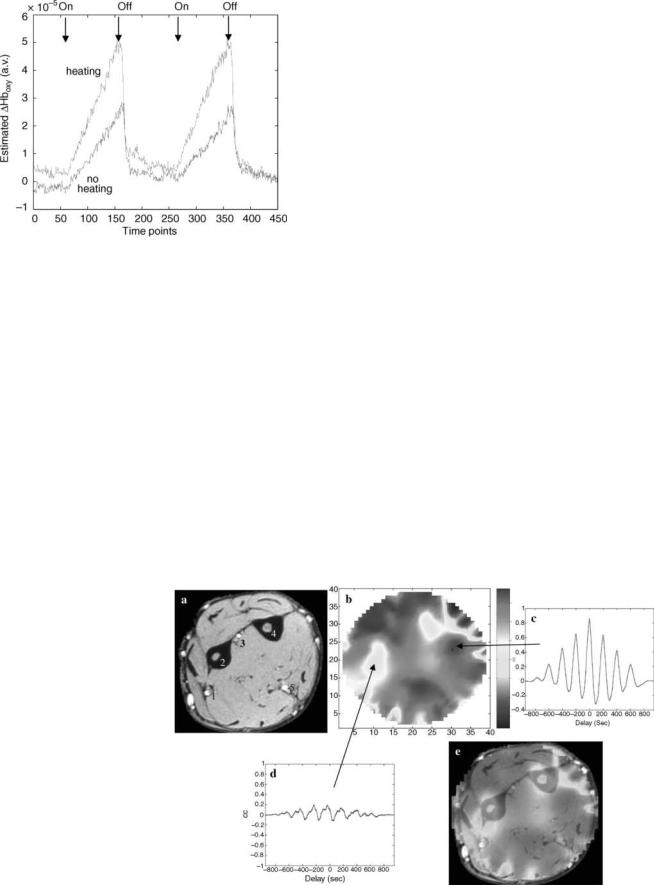
248 PERIPHERAL VASCULAR NONINVASIVE MEASUREMENTS
Figure 10. Time course of computed average oxyhemoglobin response to two cycles of mild venous occlusion in the forearm. Dark curve, no heat applied; light curve, with heat. [Reprinted with permission from R.L. Barbour et al., Functional imaging of vascular bed by dynamic optical tomography. Proceedings of SPIE, vol. 5369, in Physiology, Function, and Structure from Medical Images, 2004.]
variations in vascular density among the different tissue types, and in their responses to stimuli. Second, it also recognizes that for any given tissue, multiple response characteristics can be defined that serve to discriminate, as noted, one tissue type from another, or healthy from diseased. An example of this discriminatory capability is the following.
Shown in Fig. 10 is the response to partial cuff occlusion, applied to the arm in order to induce venous engorgement as recorded from a representative site about the forearm. Also shown is an enhanced response to a similar maneuver when the forearm was warmed by a thermal
blanket prior to the measurement. We interpret the enhanced response as evidence of a decrease in local peripheral vascular resistance due to vasodilatation. Using the response curve shown in Fig. 10, it is possible to identify where similar behavior is seen in the corresponding cross-sectional image time series. This is shown in Fig. 11, together with an MR map of the forearm for comparison to anatomy. Regions of high correlation to the response curve are seen in many areas, with distinctively lower correlation occurring in regions that correspond to the ulna and radius, a finding consistent with known differences between soft tissue and interosseous hemodynamics (see overlay in e).
Additional discriminatory information about the considered stimulus can be gleaned from other analyses of the image time series. Motivating the approach taken is knowledge that any measure of bulk tissue properties is actually a composite of multiple overlapping features due to known differences, for example, in vascular compliance attributable to the principal elements of the vascular tree (i.e., arteries, veins and microvessels). Separation of the individual components comprising the whole is attainable using a class of methods known as blind source separation techniques.
Data in Figure 12 is an example of use of these methods, applied to four consecutive mild inflation–deflation cycles of the type illustrated in Fig. 10. The dark curve corresponds to the first principal component (PC) and accounts for 80% of the signal variance. The light curve is the second PC, accounting for 10% of total variance. Inspection reveals that the time courses of the two functions differ, and that they change from one application of mild occlusion to another. In the case of the first PC, it is seen that Hboxy levels increase promptly upon inflation. Also seen is that the magnitude of this response increases modestly following the second challenge. We interpret this to represent blood volume changes in the venous
Figure 11. (a) MR cross-section of arm. (b) Cross-correlation (CC) map between (dark) model function in Fig. 10 with Hb image time series.
(c) Overlay of a and b. (d and e), Time dependence of CC at indicated locations. (1) Radial artery, (2) radius, (3) interosseous artery, (4) ulna, (5) ulnar artery. [Reprinted with permission from R.L. Barbour et al., Functional imaging of vascular bed by dynamic optical tomography. Proceedings of SPIE, vol. 5369, in Physiology, Function, and Structure from Medical Images, 2004.]
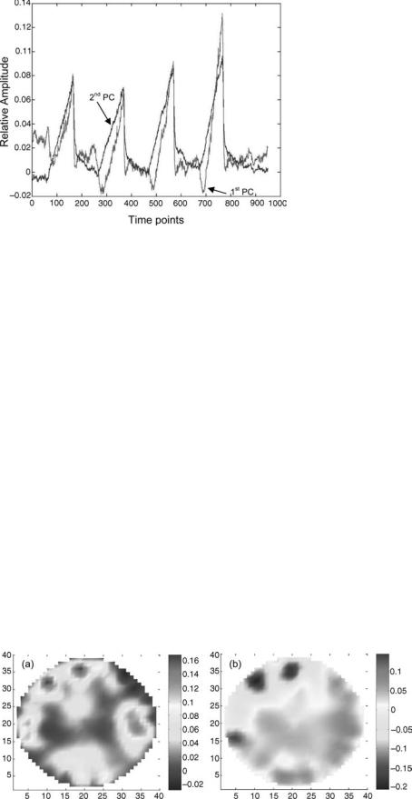
Figure 12. First (light curve) and second (dark curve) principal component (PC) of oxyhemoglobin signal computed for reconstructed image time series for four consecutive cuff inflation cycles. [Reprinted with permission from R.L. Barbour et al., Functional imaging of vascular bed by dynamic optical tomography. Proceedings of SPIE, vol. 5369, in Physiology, Function, and Structure from Medical Images, 2004.]
tree, as these distend most easily relative to the other elements of the vascular tree. The response seen in the second PC is more complex. Early on in the inflation cycle, a decline is observed, followed by an accelerated increase relative to the first PC, with proportionally greater responses upon subsequent challenges. It is believed this signal originates primarily from the microvascular bed. The initial decline in Hboxy is consistent with blood pooling, allowing for greater oxygen extraction. Following this, dilation occurs, perhaps in response to a buildup of local metabolic factors. The finding that the rate and extent of change in this signal increases in subsequent challenges suggests that insufficient time had elapsed between cycles to allow for complete washout of tissue factors. Support of this assignment is given in Fig. 13. In Fig. 13a it is seen that the signal associated with the first PC is mainly seen in the periphery (red regions), roughly in agreement with the location of near-surface veins. In contrast the signal associated with the second PC in Fig. 13b is found mainly in the ventral aspect
PERIPHERAL VASCULAR NONINVASIVE MEASUREMENTS |
249 |
of the forearm, which is dominated by well-perfused muscle.
Development of DOT technology is proceeding at a brisk pace, with new system designs being reported on a regular basis (91). As depicted here, TSI can be explored using time-series DOT. This, however, is not the only modality by which optical measures of peripheral vascular dynamics can be studied. Judging from advances made with photoacoustics (92), this approach may also prove useful (93,94). Additionally, the method could be extended further, to include use of injectable fluorescent probes or other forms of optical contrast media (95).
SUMMARY
Knowledge about the physiological and pathological state of the peripheral vasculature is extremely useful in the detection and staging of PVD, which occur with high prevalence and are associated with significant morbidity and mortality rates. Noninvasive measurements of those parameters are desirable because they can be performed more easily, are more cost effective, and are better suited for use as general screening tools than are invasive techniques. Volume-integrated dynamic flow measures can be obtained with a variety of available plethysmography methods. Measuring the flow response to occlusion maneuvers allows extraction of vessel flow and compliance values. In addition, plethysmography allows pulse volume recording in different locations on the extremities, and the interpretation of pulse wave contours and velocities permits drawing of inferences regarding peripheral, and even central, arterial health. Ultrasound methods, both structural and Doppler flow measurements, are valuable tools for diagnosing stenoses and thromboses. Laser Doppler flowmetry is a relatively new method for investigating the superficial microvessels.
Several imaging modalities are available for the assessment of blood flow and the vasculature. Most of these rely on contrast agents, and therefore can not strictly be considered noninvasive. The degree of invasiveness, however, seems small enough to justify their mentioning in the context of this article. Besides the conventional imaging methods, which include X ray CT, various MRI methods, and PET, the new noninvasive imaging technique of temporal spectral imaging, and in particular its
Figure 13. (a) Amplitude map of first principal component (PC) of total Hb (82% of total variance). (b) Amplitude map of second PC of total Hb (10% of total variance). [Reprinted with permission from R.L. Barbour et al., Functional imaging of vascular bed by dynamic optical tomography. Proceedings of SPIE, vol. 5369, in Physiology, Function, and Structure from Medical Images, 2004.]
250 PERIPHERAL VASCULAR NONINVASIVE MEASUREMENTS
implementation through diffuse optical tomography is introduced.
BIBLIOGRAPHY
Cited References
1.Drzewiecki G. Noninvasive arterial blood pressure and mechanics. Bronzino X, editor. The Biomedical Handbook. 2nd ed. Boca Raton, (FL): CRC Press and IEEE Press; 2000.
2.Penˇ a´z J. Photoelectric measurement of blood pressure, volume, and flow in the finger. Digest 10th Internation Conference Medical Biological Engineering Dresden. 1973;104.
3.Wesseling KH, Settels JJ, De Wit B. The measurement of continuous finger arterial pressure non-invasively in stationary subjects. In: Schmidt TH, Dembroski TM, Bluemchen G, etitors. Biological and Psychological Factors in Cardiovascular Disease. Berlin: Springer-Verlag; 1986.
4.Parati G, et al. Non-invasive beat-to-beat blood pressure monitoring: new developments. Blood Press Mon 2003;8:31–36.
5.Bos WJW, et al. Reconstruction of brachial artery pressure from noninvasive finger pressure measurements. Circulation 1996;94:1870–1875.
6.Pressman GL, Newgard PM. A transducer for the continuous external measurement of arterial blood pressure. IEEE Trans Biomed Eng 1963;10:73–81.
7.Scha¨fer EA, Moore B. On the contractility and innervation of the spleen. J Physiol 1896;20:1–5.
8.Hewlett AW, Zwaluwenburg JG. The rate of blood flow in the arm. Heart 1909;1:87–97.
9.Whitney RJ. The measurement of volume changes in human limbs. J Physiol 1953;121:1–27.
10.McGivern RC, et al. Computer aided screening for deep venous thrombosis. Automedica 1991;13:239–244.
11.Schu¨ rmann M, et al. Assessment of the peripheral microcirculation using computer-assisted venous congestion plethysmography in post-traumatic complex regional pain syndrome type I. J Vasc Res 2001;38:453–461.
12.Leslie SJ, et al. Comparison of two plethysmography systems in assessment of forearm blood flow. J Appl Physiol 2004;96: 1794–1799.
13.Nyboer J, Bango S, Barnett A, Halsey RH. Radiocardiograms - the electrical impedance changes of the heart in relation to electrocardiograms and heart sounds. J Clin Invest 1940; 19:773.
14.Nyboer J. Regional pulse volume and perfusion flow measurements: Electrical impedance plethysmography. Arch Int Med 1960;105:264–276.
15.Nybor J. Electrical Impedance Plethysmography. 2nd ed, Springfield, (IL): Charles C Thomas; 1970.
16.Malmivuo J, Plonsey R. Bioelectromagnetism—Principles and Applications of Bioelectric and Biomagnetic Fields. New York: Oxford University Press; 1995.
17.Patterson R. Bioelectric impedance measurements. Bronzino X, editor. The Biomedical Handbook. 2nd ed, Boca Raton, (FL): CRC Press and IEEE Press; 2000.
18.Hertzman AB. Photoelectric plethysmography of the fingers and toes. Proc Soc Exp Biol Med 1937;37:529–534.
19.Hielscher AH, et al. Sagittal laser optical tomography for imaging of rheumatoid finger joints. Phys Med Biol 2004;49: 1147–1163.
20.De Trafford J, Lafferty K. What does photoplethysmography measure?. Med Biol Eng Comput 1984;22(5):479–480.
21.Jespersen LT, Pedersen OL. The quantitative aspect of photoplethysmography revised. Heart Vessels 1986;2:186– 190.
22.Kamal AA, Harness JB, Irving G, Mearns AJ. Skin photoplethysmography — a review. Comput Methods Programs Biomed 1989;28(4):257–269.
23.Hashimoto J, et al. Pulse wave velocity and the second derivative of the finger photoplethysmogram in treated hypertensive patients: their relationship and associating factors. J Hypertens 2003;20(12):2415–2422.
24.Millasseau SC, et al. Noninvasive assessment of the digital volume pulse — Comparison with the peripheral pressure pulse. Hypertension W 2000;20(12):2415–2422.
25.Webb A. Introduction to Biomedical Imaging. Hoboken, (NJ): John Wiley & Sons Inc.; 2003.
26.Halpern JL. Evaluation of patients with peripheral vascular disease. Thrombosis Res 2002;106:V303–V311.
27.Hirsch AT, et al. Peripheral arterial disease detection, awareness, and treatment in primary care. JAMA 2001;286:317– 1324.
28.Hooi JD, et al. Risk factors and cardiovascular diseases associated with asymptomatic peripheral arterial occlusive disease. The Limburg PAOD Study. Peripheral Arterial Occlusive Disease. Scand J Prim Health Care 1998;16(3): 177–182.
29.Weitz JI, et al. Diagnosis and treatment of chronic arterial insufficiency of the lower extremities: A critical review. Circulation 1996;94:3026–3049.
30.Carman TL, Fernandez BB. A primary care approach to the patient with claudication, Phys Am Fam 2000;61: 1027–1032. 1034.
31.Holland T. Utilizing the ankle brachial index in clinical practice. Ostomy Wound Manage 2002;48(1):38–40, 43–46, 48–49.
32.Sacks D, et al. Position statement on the use of the ankle brachial index in the evaluation of patients with peripheral vascular disease — A consensus statement developed by the standards division of the Society of Interventional Radiology. J Vasc Interv Radiol 2003;14:S389.
33.Donnelly R, Hinwood D, London NJM. ABC of arterial and venous disease: Non-invasive methods of arterial and venous assessment. studentBMJ 2000;8:259–302.
34.Vascular Technology Professional Performance Guideline — Lower Extremity Arterial Segmental Physiologic Evaluation, Society for Vascular Ultrasound; 2003.
35.Rietzschel E-R, et al. A comparison between systolic and diastolic pulse. Hypertension 2001;37:e15–e22.
36.Frank O. Die Grundform der Arteriellen Pulses. Acta Biol 1899;37:426–483.
37.Cohn JN, et al. Noninvasive pulse wave analysis for the early detection of vascular disease. Hypertension 1995;26:503– 508.
38.Millasseau SC, Kelly RP, Ritter JM, Chowienczyk PJ. Determination of age-related increases in large artery stiffness by digital pulse contour analysis. Clin Sci 2002;103: 371–377.
39.Lekakis JP, et al. Arterial stiffness assessed by pulse wave analysis in essential hypertension: relation to 24-h blood pressure profile. Int J Cardiol 2005;102:391–395.
40.O’Rourke MF, Gallagher DE. Pulse wave analysis. J Hypertens Suppl 1996;14(5):S147–157.
41.Tsai W-C, et al. Association of risk factors with increased pulse wave velocity detected by a novel method using dualchannel photoplethysmography. Am J Hyper 2005;18:1118– 1122.
42.Nigam A, Mitchell GF, Lambert J, Tardif J-C. Relation between conduit vessel stiffness (assessed by tonometry) and endothelial function (assessed by flow-mediated dilatation) in patients with and without coronary heart disease. Am J Cardiol 2003;92:395–399.
43.O’Rourke MF, Adji AA. An updated clinical primer on large artery mechanics: implications of pulse waveform analysis and arterial tonometry. Curr Opin Cardiol 2005;20(4): 275–81.
44.Gamble J, Gartside IB, Christ F. A reassessment of mercury in silastic strain gauge plethysmography for microvascular permeability assessment in man. J Physiol 1993;464: 407–422.
45.Maskell NA, et al. The use of automated strain gauge plethysmography in the diagnosis of deep vein thrombosis. Br J Radiol 2002;75:648–651.
46.Vigilance JE, Reid HL. Venodynamic and hemorheological variables in patients with diabetes mellitus. Arc Med Res 2005;36:490–495.
47.Goddard AJP, Chakraverty S, Wright J. Computer assisted strain-gauge plethysmography is a practical method of excluding deep venous thrombosis. Clin Radiol 2001;56: 30–34.
48.Larsson M, Nilsson H, Stro¨mberg T. In vivo determination of local skin optical properties and photon path length by use of spatially resolved diffuse reflectance with applications in laser Doppler flowmetry. Appl Opt 2003;42(1):124–134.
49.Bonner R, Nossal R. Model for laser Doppler measurements of blood flow in tissue. Appl Opt 1981;20(20):2097–2107.
50.Serov A, Lasser T. High-speed laser Doppler perfusion imaging using an integrating CMOS image sensor. Opt Expr 2005;13(17):6416–6428.
51.Freccero C, et al. Laser Doppler perfusion monitoring of skin blood flow at different depths in finger and arm upon local heating. Microvasc Res 2003;66:183–189.
52.Eskandary H, Shahabi M, Asadi AR. Evaluation of carpal tunnel syndrome by laser Doppler flowmetry. Iran J Med Sci 2002;27(2):87–89.
53.Scharf A, et al. Evaluation of two-dimensional versus threedimensional ultrasound in obstetric diagnostics: A prospective study. Fetal Diag Ther 2001;16:333–341.
54.Zotz RJ, Trabold T, Bock A, Kollmann C. In vitro measurement accuracy of three-dimensional ultrasound. Echocardiography 2001;18:149–56.
55.Hoksbergen AWJ, et al. Success rate of transcranial colorcoded duplex ultrasonography in visualizing the basal cerebral arteries in vascular patients over 60 years of age. Stroke 1999;30:1450–1455.
56.Fu¨ rst G, et al. Reliability and validity of noninvasive imaging of internal carotid artery pseudo-occlusion. Stroke 1999;30: 1444–1449.
57.Rubin JM, et al. Power Doppler US: a potentially useful alternative to mean frequency-based color Doppler US. Radiology 1994;190:853–856.
58.Steinke W, et al. Power Doppler imaging of carotid artery stenosis: Comparison with color Doppler flow imaging and angiography. Stroke 1997;28:1981–1987.
59.Blomley MJK, et al. Liver microbubble transit time compared with histology and Child-Pugh score in diffuse liver disease: a cross sectional study. Gut 2003;52:1188–1193.
60.Della Martina A, Meyer-Wiethe K, Alle´mann E, Seidel G. Ultrasound contrast agents for brain perfusion imaging and ischemic stroke Therapy. J Neuroimaging 2005;15: 217–232.
61.Rofsky NM, Adelman MA. MR angiography in the evaluation of atherosclerotic peripheral vascular disease. Radiology 2000;214:325–338.
62.Baumgartner I, et al. Leg ischemia: Assessment with MR angiography and spectroscopy. Radiology 2005;234:833–841.
63.Kucharczyk W, et al. Intracranial lesions: flow-related enhancement on MR images using time-of-flight effects. Radiology 1986;161:767–772.
PERIPHERAL VASCULAR NONINVASIVE MEASUREMENTS |
251 |
64.Whittemore AR, Bradley WG, Jinkins JR. Comparison of cocurrent and countercurrent flow-related enhancement in MR imaging. Radiology 1989;170:265–271.
65.Cebral JR, et al. Blood-flow models of the circle of Willis from magnetic resonance data. J Eng Math 2003;47:369– 386.
66.Fatouraee N, Amini AA. Regularization of flow streamlines in multislice phase-contrast MR imaging. IEEE Trans Med Imag 2003;22:699–709.
67.Thomas DL, et al. The measurement of diffusion and perfusion in biological systems using magnetic resonance imaging. Phys Med Biol 2000;45:R97–R138.
68.Sorensen AG, et al. Hyperacute stroke: Simultaneous measurement of relative cerebral blood volume, relative cerebral blood flow, and mean tissue transit time. Radiology 1999;210:519–527.
69.Wang J, et al. Arterial transit time imaging with flow encoding arterial spin tagging (FEAST). Mag Reson Med 2003;50:599– 607.
70.Mandeville JB, Marota JJA. Vascular filters of functional MRI: Spatial localization using BOLD and CBV contrast. Mag Reson Med 1999;42:591–598.
71.Ogawa S, Menon RS, Kim S-G, Ugurbil K. On the characteristics of functional magnetic resonance imaging of the brain. Annu Rev Biophys Biomol Struct 1998;27:447–474.
72.Lerman LO, Rodriguez-Porcel M, Romero JC. The development of x-ray imaging to study kidney function. Kidney Inte 1999;55:400–416.
73.Romero JC, Lilach LO. Novel noninvasive techniques for studying renal function in man. Semi Nephrol 2000;20:456– 462.
74.Gobbel GT, Cann CE, Fike JR. Measurement of regional cerebral blood flow using ultrafast computed tomography: Theoretical aspects. Stroke 1991;22:768–771.
75.Horn P, et al. Xenon-induced flow activation in patients with cerebral insult who undergo xenon-enhanced CT blood flow studies. AJNR Am J Neuroradiol 2001;22:1543–1549.
76.Matsuda M, et al. Comparative study of regional cerebral blood flow values measured by Xe CT and Xe SPECT. Acta Neurolog Scand 1996;166:13–16.
77.Yonas H, et al. Side effects of xenon inhalation. J Comput Assist Tomogr 1981;5:591–592.
78.Roberts HC, et al. Multisection dynamic CT perfusion for acute cerebral ischemia: The ‘‘toggling-table’’ technique. AJNR Am J Neuroradiol 2001;22:1077–1080.
79.Ro¨ther J, et al. Hemodynamic assessment of acute stroke using dynamic single-slice computed tomographic perfusion imaging. Arch Neurol 2000;57:1161–1166.
80.Compare, for example, the corporate web pages http:// www.anzai-med.co.jp/eigo/Xe-Per.htm and http://www.gehealthcare.com/usen/ct/case_studies/products/perfusion.html, which assert superiority for the Xeand I-based approaches, respectively. One apparent reason for disagrement is the issue of the relative contributions to the image of the blood vessels’ walls and of their contents.
81.Bambakidis NC, et al. Functional evaluation of arteriovenous malformations. Neurosurg Focus 2001;11: Article 2.
82.Schaefer WM, et al. Comparison of microsphere-equivalent blood flow (15O-water PET) and relative perfusion (99mTctetrofosmin SPECT) in myocardium showing metabolism-per-
fusion mismatch. J Nucl Med 2003;44:33–39.
83. Barbour RL, et al. Functional imaging of the vascular bed by dynamic optical tomography. Proc SPIE 2004;5369: 132–149.
84.Barbour RL, Lubowsky J, Graber HL. Use of reflectance spectrophotometry (RS) as a possible 3-dimensional (3D) spectroscopic imaging technique. FASEB J 1988;2:A 1772.