

72 NUCLEAR MAGNETIC RESONANCE SPECTROSCOPY
of Ultrasound in Obstetrics and Gynecology (ISUOG). Ultrasound Obstet Gynecol 2003;21:100.
11.Safety statement, 2000. International Society of Ultrasound in Obstetrics and Gynecology (ISUOG). Ultrasound Obstet Gynecol 2000;16:594–596.
12.Hocking B, Joyner KJ, Newman HH, Aldred RJ. Radiofrequency electric shock and burn. Med J Aust 1994;161:683–685.
13.Schilling CJ. Effects of exposure to very high frequency radiofrequency radiation on six antenna engineers in two separate incidents. Occup Med (Lond) 2000;50:49–56.
Further Reading
Australian Radiation Protection and Nuclear Safety Agency: http://www.arpansa.gov.au
Dennis JA, Stather J, editors. Non-ionizing radiation. Radiation Protection Dosimetry. 1997. 72:161–336.
ICNIRP references from Health Physics: http://www.icnirp.de. National Radiological Protection Board (NRPB) U.K.: http://
www.nrpb.co.uk.
See also BIOMATERIALS, SURFACE PROPERTIES OF; IONIZING RADIATION,
BIOLOGICAL EFFECTS OF; RADIATION THERAPY SIMULATOR.
NUCLEAR MAGNETIC RESONANCE
IMAGING. See MAGNETIC RESONANCE IMAGING.
NUCLEAR MAGNETIC RESONANCE
SPECTROSCOPY
WLAD T. SOBOL
University of Alabama
Birmingham, Alabama
INTRODUCTION
When two independent groups of physicists (Bloch, Hansen, and Packard at Stanford and Purcell, Torrey, and Pound at MIT) discovered the phenomenon of nuclear magnetic resonance (NMR) in bulk matter in late 1945, they already knew what they were looking for. Earlier experiments by Rabi on molecular beams, and the attempts of Gorter to detect resonant absorption in solid LiF, seeded the idea of NMR in bulk matter. Fascinating stories describing the trials and tribulations of the early developments of NMR concepts have been told by several authors, but Becker et al. (1) deserve a special citation for the completeness of coverage.
For his achievements, Rabi was awarded a Nobel Prize in 1944, while Bloch and Purcell jointly received theirs in 1952. What was the importance of the Bloch and Purcell discoveries to warrant a Nobel Prize despite an abundance of prior work offering numerous clues? It was not the issue of special properties of elementary particles, such as a spin or magnetic moment: This was first demonstrated by the Stern–Gerlach experiment. It was not the issue of the particle interactions with magnetic field: This was first illustrated by the Zeeman effect. It was not even
the magnetic resonance phenomenon itself: This was first demonstrated by Rabi. It was the discovery of a tool that offered a robust, nondestructive way to study the dynamics of interactions in bulk matter at the atomic and molecular level that forms the core of Bloch and Purcell’s monumental achievements. However, despite the initial excitement at the time of their discovery, no one could have predicted just how extensive and fruitful the applications of NMR would turn out to be.
What is the NMR? The answer depends on who you ask. For Bloch’s group at Stanford, the essence of magnetic resonance was a flip in the orientation of magnetic moments. Bloch conceptual view of the behavior of the nuclear magnetic moments associated with nuclear spins was, in essence, a semiclassical one. When a sample substance containing nuclear spins was kept outside a magnetic field, the magnetic moments of individual spins were randomly oriented in space, undergoing thermal fluctuations (Brownian motion). The moment the sample was placed in a strong, static magnetic field, quantum rules governing the behavior of the spins imposed new order in space: the magnetic moments started precessing around the axis of the main magnetic field. For spin ½ particles (e.g., protons), only two orientations w.r.t. static magnetic field were allowed; thus some spins precessed while oriented somewhat along the direction of the external field, while other spun around while orienting themselves somewhat opposite to the direction of that field. To Bloch, a resonance occurred when externally applied radio frequency (RF) field whose frequency matched the precessional frequency of the magnetic moments, forced a reorientation of precessing spins from parallel to antiparallel (or vice versa). They called this effect a nuclear induction.
As far as the Purcell’s group was concerned, NMR was a purely quantum mechanical phenomenon. When a diamagnetic solid containing nuclei of spin I is placed in a static magnetic field, the interactions of nuclear magnetic moments with the external magnetic field cause the energy levels of the spin to split (the anomalous Zeeman effect). When an external RF field is applied, producing quanta of energy that match the energy difference between the Zeeman levels, the spin system would absorb the energy and force spin transitions between lower and upper energy states. Thus, they described the phenomenon as resonance absorption.
It can be proven that these two concepts of NMR phenomenon are scientifically equivalent. However, the two views are psychologically very different, and have been creating a considerable chasm in the accumulated body of knowledge. Some aspects of NMR applications are intuitively easier to understand using Bloch’s semiclassical vector model, while other naturally yield themselves to the quantum picture of spin transitions among energy states. The details of this dichotomy and its impact on the field of NMR applications are fascinating by themselves and have been extensively discussed by Ridgen (2).
At the time of the NMR discovery, nobody had any inkling that this phenomenon might have any applications in medicine. To understand how NMR made such a big impact in the medical field, one has to examine how the NMR and its applications evolved in time. Nuclear mag-
netic resonance was discovered by physicists. Thus it is not surprising that the initial focus of the studies that followed was on purely physical problems, such as the structure of materials and dynamics of molecular motions in bulk matter. During a period of frenzied activities that followed the original reports of the discovery, it was very quickly understood that interactions among nuclear spins, as well as the modification of their behavior by the molecular environment, manifest themselves in two different ways. On the one hand, the Zeeman energy levels could shift due to variations in the values of local magnetic field at different sites of nuclear spins within the sample. This causes the resonant absorption curve to acquire a fine structure. Such studies of NMR lineshapes provide valuable insights into the structure and dynamics of molecular interactions, especially in crystals. This branch of NMR research is customarily referred to as radiospectroscopy.
On the other hand, when a sample is placed in the external magnetic field, the polarization of spin orientations causes the sample to become magnetized. When the sample is left alone for some time, an equilibrium magnetization develops. This equilibrium magnetization, M0, is proportional to the strength and aligned in the direction of the external static magnetic field, B0. An application of RF field disturbs the equilibrium and generally produces a magnetization vector, M, that is no longer aligned with B0 . When the RF field is switched off, the magnetization returns over time to its equilibrium state; this process is called a relaxation. The process of restoring the longitudinal component of the equilibrium magnetization requires that the spins exchange energy with their environment; thus, it is commonly referred to as spin–lattice or longitudinal relaxation. The characteristic time that quantifies the rate of recovery of the longitudinal component of magnetization toward its equilibrium value, M0, is called the spin–lattice relaxation time and denoted T1 or, in medical applications, T1. At equilibrium, the transverse magnetization component is zero. Thus, any nonzero transverse component of nonequilibrium magnetization must decay back to zero over time. This process tends to be dominated by interactions among spins and is thus called a spin–spin or transverse relaxation. The characteristic time that quantifies the rate of decay of the transverse component of magnetization is called the spin–spin relaxation time and denoted T2 or, in medical applications, T2. Both T1 and T2 strongly depend on the nature of the molecular environment within which the spins are immersed, thus offering a robust probe of molecular dynamics and structure in a variety of materials (solid, liquid, and gaseous) over a range of conditions (temperature, phase transitions, chemical reactions, translational and rotational diffusion, etc.). Studies of relaxation times are referred to simply as NMR relaxation studies, and sometimes as relaxometry.
In solids, dipole–dipole interactions among spins are dominant, which for proton NMR (1H NMR) studies results in fairly wide lineshapes (with a width of several kHz) with very little fine structure. In most liquids, however, the substantially faster molecular reorientations average the dipole–dipole interactions, effectively suppressing them to
NUCLEAR MAGNETIC RESONANCE SPECTROSCOPY |
73 |
produce a vanishing net effect on the NMR absorption curves that become much narrower (typically of the order of Hz). This feature has led to a discovery of chemical shift phenomenon.
The most dramatic demonstration of the chemical shift was the observation made in 1951 by Arnold et al. (3) who showed separate spectral NMR lines from nonequivalent protons in a sample containing a simple organic substance, ethanol. This gave birth to high-resolution NMR spectroscopy or HR NMR, a powerful tool that assists chemists in nondestructive analysis of organic compounds. This in vitro technique underwent massive developments over the years and almost overshadowed the NMR applications in physics. An exhaustive overview of HR NMR applications has been published by Shoolery (4). Today, HR NMR spectroscopy plays a major role in studies of biological materials in vitro and in drug development research. This research, although not directly used in clinical care, nevertheless is having a major impact on the development of medical arts. A comprehensive review of biological applications of NMR spectroscopy has been provided by Cohen et al. (5).
Standard NMR studies are performed in vitro: The sample is placed in the bore of a laboratory magnet, and the signal is collected from the entire volume of the sample. Samples are relatively small: The typical NMR tube vial is5 mm outside diameter (OD) and holds 0.5 mL of sample material. Nuclear magnetic resonance magnets have relatively small active volumes [typical bore size of modern NMR cryomagnets is 70 mm inside diameter
(ID)], but very high magnetic field homogeneity, routinely > 10 9 B0.
In the early 1970s, a revolutionary concept emerged from the pioneering work of Lauterbur in the United States and Mansfield, Andrew, and Hinshaw in the United Kingdom. They discovered that by using judiciously designed magnetic field gradients it was possible to retrieve an NMR signal from a small localized volume (called a voxel) within a much larger sample (e.g., a human body). This started a new field of NMR applications, called magnetic resonance imaging (MRI) that greatly enhanced the practice of diagnostic medicine (see the section Magnetic Resonance Imaging).
One of the frustrating limitations of MRI applications was the ambiguity of lesion characterization. The development of MRI focused on the noninvasive visualization of soft tissues within the living human body; as a result, the technical and engineering trade-offs made in the process of improving the quality of images have essentially rendered the method nonquantitative. In essence, MRI proved to be extremely sensitive in the detection of various lesions within the patient’s body, but not very robust in providing information needed to fully identify the characteristics of the tissue within the lesion. Thus, in addition to basic NMR tissue characteristics (proton density, T1, and T2), the interpreters of medical MR images came to rely on morphology of lesions (size, shape, and location) to draw conclusions about lesion pathology. In this context, the concept of localized NMR spectroscopy experiments, where MRI techniques are used to locate the lesion and localize the volume of interest, while NMR spectroscopic techniques are used to acquire NMR spectra of the tissue within a lesion, becomes intuitively
74 NUCLEAR MAGNETIC RESONANCE SPECTROSCOPY
evident. However, while the concept may appear naturally obvious, implementations have proven to be extremely difficult. Despite first successful experiments in acquiring localized phosphorus 31P NMR in vivo spectra from a human forearm, performed in 1980 by a group led by Chance, the true clinical applications of localized NMR spectroscopy have only recently begun to appear. While first attempts focused on 31P NMR spectroscopy using surface coils to localize the signals within the human body, current clinical applications almost exclusively utilize 1H NMR spectra to gain additional, clinically relevant information about the lesion of interest. The methodology used in this approach is referred to as magnetic resonance spectroscopy (MRS), magnetic resonance spectroscopic imaging (MRSI), or chemical shift imaging (CSI). Techniques of this particular application of the NMR phenomena in medical practice will be the subject of further discussion here. While the interest in exploring clinical applications of MRS of nuclei other than protons (e.g., 31P, 13C, 19F, and 23Na) still remains, a vast majority of current clinical applications uses 1H MRS and thus only this particular nucleus will be considered in further discourse. Readers interested in other nuclei are encouraged to explore literature listed in the Reading List section.
THEORY
In this section, the quantum mechanical approach of formalism is used, since this formalism is most naturally suited to explain the various features of NMR spectra. To begin with, consider an ensemble of noninteracting protons, free in space where a strong, perfectly uniform magnetic field B0 is present. Because all spins are considered identical, the Hamiltonian of the system includes a single spin and all quantum mechanical expectation values are calculated over the entire assembly of spins. Under those conditions, the Hamiltonian (H) describes the Zeeman interaction of the nuclear magnetic moment m with the external magnetic field and has a form
H ¼ m B0 ¼ ghB0Iz |
(1) |
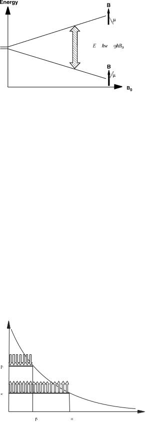
where g is the gyromagnetic ratio, h is the Planck’s constant, and Iz is the z component of the nuclear spin operator I, which for protons has an eigenvalue value of ½. Because Iz has only two eigenvalues, ½, the system’s ground energy level is split into two sublevels, with the energy gap proportional to B0, as shown in Fig. 1. Now assume that spins are allowed to weakly interact with their molecular environment, which are collectively described as the lattice (regardless of the actual state of the sample; e.g., in liquids the lattice refers to thermal diffusion, both rotational and translational, of the atoms or molecules that host the spins). When the system is left undisturbed over time, it will reach a thermal equilibrium, where the spin populations at the higher and lower energy levels are described by a Boltzmann distribution, as shown in Fig. 2. The resultant sample equilibrium magnetization is equal to
Figure 1. The Zeeman splitting of the ground-state energy levels for the spin ½ system as a function of the external magnetic field strength, B0.
where T is the absolute temperature of the sample, N is a number of spins in the sample, and k is the Boltzmann constant. At normal conditions, this equilibrium magnetization is too small to be detectable, but when a resonance phenomenon is exploited by applying a short burst of RF energy at resonance frequency v0 (called an RF pulse), the magnetization can be flipped onto a transverse plane, perpendicular to the direction of B0. This transverse magnetization will precess at the resonant frequency of the spins and thus will generate an oscillating magnetic field flux in the receiver coils of the NMR apparatus, which will be detected as a time-varying voltage at the coils terminals. This signal is called a free induction decay (FID) and its time evolution contains information about the values of resonant frequency of the spins, v0, the spinspin relaxation time, T2, and the distribution of local static magnetic fields at the locations of the spins, T2 . The local static magnetic fields, experienced by spins at different locations in the sample, may vary from spin site to spin site, chiefly due to the inhomogeneity of the main magnetic field B0. In addition, in heterogeneous samples, commonly encountered in in vivo experiments, local susceptibility variations may contribute to T2 effects. For a variety of reasons, the chief one being the ease of
Energy
E
E
N |
N |
Population |
eq |
¼ M0 ¼ |
g2h2NB0 |
(2) |
Figure 2. An illustration of Boltzmann distribution of spin |
Mz |
4kT |
populations for an ensemble of identical spins ½, weakly |
||
|
|
|
|
interacting with the lattice, at thermal equilibrium.
y '
t
x ' |
FID (Free Induction Decay) |
|
t
Figure 3. Real and imaginary components of an FID signal.
interpretation, the FID signal is always recorded in the reference frame that rotates at the frequency v close to v0, (called ‘‘the rotating frame’’). From the engineering point of view, recording the signal in the reference frame, rotating at the frequency v, is equivalent to frequency demodulation of the signal by frequency v.
The recorded FID has two components: one, called real, or in-phase, is proportional to the value of transverse spin magnetization component aligned along the y’ axis of the rotating frame (the [x’, y’, z] notation is used to denote rotating frame, as opposed to the stationary, laboratory frame [x, y, z]). The other FID component is proportional to the value of transverse spin magnetization projected along the x’ axis and is referred to as imaginary, or out-of-phase signal (see Fig. 3). To a human being, the FID signals can be difficult to interpret; thus an additional postprocessing step is routinely employed to facilitate data analysis. A Fourier transform (FT) is applied to the FID data and the signal components having different frequencies are retrieved, producing an NMR spectrum (see Fig. 4).
The chemical shift, mentioned earlier, is responsible for a plethora of spectral lines (peaks) seen in a typical NMR spectrum. Consider a simple organic molecule that contains hydrogen localized at three nonequivalent molecular sites. Chemists call molecular sites equivalent if the structure of chemical bonds around the site creates an identical distribution of electron density at all proton locations. When the sites are nonequivalent, different distributions of electron cloud around the protons will have a different shielding effect on the value of the local magnetic field, experienced by individual protons. The strength of electron shielding effect is proportional to the value of B0 and is accounted for in the Hamiltonian by using a shielding constant, s.
3 |
|
|
˚ |
siÞB0Izi |
(3) |
H ¼ ghi a1ð1 |
||
¼ |
|
|
In this example, a molecule with only three nonequivalent
NUCLEAR MAGNETIC RESONANCE SPECTROSCOPY |
75 |
y '
Real
|
|
|
|
t |
x ' |
|
|
FID |
|
|
|
|
|
|
|
|
|
|
Time |
|
|
|
|
t |
|
|
Imaginary |
FT |
|
|
|
|
|
|
|
SPECTRUM |
|
Frequency |
|
|
Real |
|
|
|
5.0 |
4.0 |
3.0 |
2.0 |
1.0 |
|
|
ppm |
|
|
Figure 4. A method of generating an NMR spectrum from the FID signals.
proton sites has been considered; in general, the summation index in Eq. (3) must cover all nonequivalent sites, however, many may be present. It is evident from Eq. (3) that individual protons located at different sites will have slightly different resonant frequencies, which will give rise to separate resonant peaks located at different frequencies in the observed NMR spectrum, as shown in Fig. 4. This accounts for a fine structure of NMR spectra that consists of multiple lines at different frequencies, identifying all nonequivalent molecular sites in the sample studied.
The interaction of the nuclear spin with the electron cloud surrounding it has a feedback effect, resulting in a slight distortion of the cloud; the degree of this alteration is different depending on whether the spin is up or down w.r.t. the magnetic field B0. This distortion has a ripple effect on surrounding nonequivalent spins, and consequently they become coupled together via their interactions with the electron cloud; this phenomenon is called a spin–spin coupling or J coupling, and is accounted for by adding another term to the spin Hamiltonian:
|
n |
e´ |
|
|
|
|
|
|
|
|
|
|
|
|
|
u` |
|
|
H ¼ i |
a˚ |
eˆgh |
1 |
|
s |
iÞ |
B |
I |
a˚ |
J |
I |
i |
I |
j |
u´ |
(4) |
||
¼ |
1 e¨ |
ð |
|
|
0 |
|
zi þ j < i |
|
i j |
|
uˆ |
|
||||||
|
|
|
|
|
|
|
|
|
|
|
|
|
|
|
|
|
|
|
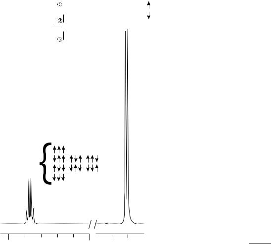
where Jij, known as a spin–spin coupling constant, describes the strength of this effect for each pair of nonequivalent protons. The presence of spin–spin coupling leads to a hyperfine structure of the NMR spectra, splitting peaks into multiplet structures, as shown in Fig. 5 that contains two fragments of an NMR spectrum of lactic acid. The structure of each multiplet can be explained using simple arrow diagrams, visible next to NMR lines. The signal at 1.31 ppm is generated by 3 equiv protons located in the CH3 group that are linked to the proton spin in the CH group via J coupling. The spin of the proton in the CH group can have only two orientations: up or down, as indicated by arrows
76 NUCLEAR MAGNETIC RESONANCE SPECTROSCOPY
Coupling constant
Amplitude
Linewidth
Reference peak
Intensity (area)
Chemical shift
Figure 5. A fragment of experimental spectrum (lactic acid at 500 MHz) showing resonances from a CH3 group (at 1.31 parts per million, ppm) and a CH group (at 4.10 ppm), respectively. The splitting of CH3 resonance into a doublet and the CH resonance into a quadruplet is caused by the J coupling. The structure of each multiplet can be derived using simple rule of grouping spins according to their orientations, as shown by groups of arrows.
that follow the bracket next to the CH3 label. Thus, the signal from CH3 protons is expected to split into a doublet with relative signal intensities 1:1, as indeed is seen in the recorded spectrum. Similarly, the signal at 4.10 ppm is generated by a single proton in the CH group that is linked via J coupling to 3 equiv protons in the CH3 group. The spins within this group of three protons can assume eight different configurations, depending on their orientation w.r.t. to the magnetic field B0. Some of those orientations are equivalent (i.e., they have the same energy) and thus can be lumped together, as shown by groups of arrows that follow the bracket next to the CH label. Simple counting leads to a prediction that the signal from the CH proton should split into a quadruplet with relative signal intensities 1:3:3:1. Again, this is clearly visible in the recorded spectrum.
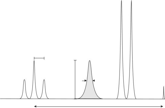
As illustrated in Fig. 6, these simple considerations show that each peak in the spectrum can be fully characterized by specifying its position w.r.t. an established reference peak (chemical shift), amplitude, intensity (intensity, or the area under the peak, is proportional to the concentration of spins contributing to the given peak), linewidth (provides information T2 and magnetic field homogeneity), and multiplet structure (singlet, doublet, triplet, etc., carries information about J coupling). Thus, the NMR spectra, like the one in Fig. 4 showing an experimental spectrum of vegetable (maize) oil, contain a wealth of information about the structure and conformation of molecules found within the sample.
Strictly speaking, the linewidths of the peaks in the NMR spectrum are determined by the values of T2 and thus are sensitive to the homogeneity of the main magnetic field and other factors contributing to the distribution of local static magnetic fields seen by the spins. Wider distributions of local fields, lead to shorter T2 values and broader corresponding peaks in the NMR spectrum. Broad peaks make spectra harder to interpret due to overlap between peaks located close to each other. This feature puts a premium on shimming skills of the NMR spectrometer operator (shimming includes methods to improve the homogeneity of the static magnetic field). For in vivo studies, the shimming tasks are made even more difficult by tissue heterogeneity that causes local variations in the magnetic field (referred to as susceptibility effects within the MRS community).
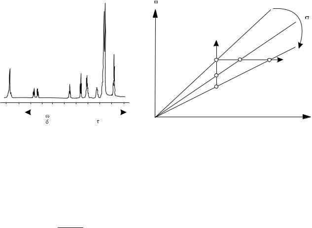
There is a peculiar feature in the way the NMR spectra are recorded that routinely confounds the NMR newbies. For historical reasons, the NMR spectra are plotted as if the spectrometer frequency was kept constant and the magnetic field B0 was varied (swept) over a range of values to record all the characteristic peaks (see Fig. 7a). In this approach, the horizontal axis of the plot represents the values of the external magnetic field necessary to reach a resonant condition for a given group of spins. However, all modern NMR spectrometers use an acquisition method in which the magnetic field B0 is kept constant and differences in resonant frequencies of various nuclei (due to their
COO*H CH3
OH CH
CH3
CH
4.5 |
4.0 |
1.5 |
|
(ppm) |
|
Figure 6. A |
schematic representation |
illustrating various |
characteristic parameters used to describe elements of an NMR spectrum.
diverse chemical shifts) are recorded instead. It is fundamental to understand that if the horizontal axis of an NMR spectrum was meant to represent the resonant frequencies of nuclei with different chemical shift, all residing in the same external magnetic field B0, then the lines to the right would represent signals with lower frequencies, which at best is counterintuitive. This paradox is resolved when one looks at the relationship between magnetic field and NMR resonance frequency for nuclei located at sites with varying electron shielding. This relationship is derived from Eq. (3), leading to the well–known Larmor equation:
w ¼ gð1 sÞB0 |
(5) |
This equation is plotted in Fig. 7b for three sites with different values of the chemical shielding constant s. As s increases, the slope of the line decreases. Thus, if the RF frequency is kept constant and the magnetic field is swept to reach subsequent resonant conditions, the weakly shielded nuclei will resonate at lower field, and as the strength of the shielding effect increases, the external
NUCLEAR MAGNETIC RESONANCE SPECTROSCOPY |
77 |
magnetic field must be increased to compensate for the increased shielding. It must be reiterated that the term magnetic field used in this context refers to the external magnetic field B0, produced by the spectrometer’s magnet, and not to the value of the local magnetic field that the spin is actually experiencing. Therefore, the signals from heavily shielded nuclei will appear at the high end of the spectrum, as illustrated by the horizontal line in Fig. 7b. On the other hand, if the external magnetic field B0 is kept constant and the frequency content of the FID signal is looked at, it will be noticed that nuclei at heavily shielded sites resonate at lower frequency, which reflects the decrease of the local magnetic field due to the shielding effects. Therefore, the signals from heavily shielded nuclei will appear at the low end of the spectrum, as illustrated by the vertical line in Fig. 7b. Historically, magnetic field sweeping was used in the early days of NMR spectroscopy and a sizeable volume of reference spectra were all plotted using the fixed-frequency convention. This standard was retained after pulsed NMR technology replaced the earlier continuous wave NMR spectroscopy, despite the fact that the fixed-field approach would have been far more natural.
The size of the chemical shift varies linearly with the strength of the magnetic field B0, which makes comparison of spectra acquired with NMR spectrometers working at different field strengths a chore. To simplify matters, chemists introduced a concept of relative chemical shift, which is defined as follows: It is realized that the term v in Eq. 5 represents a resonant frequency of a group of equivalent spins in their local magnetic field, BL. Thus, Eq. (5) can be used to define a variable t as
t |
¼ |
s |
|
106 |
¼ |
BL B0 |
|
106 |
(6) |
|
B0 |
||||||||||
|
|
|
|
|
The value of t is dimensionless and expresses the value of the shielding constant s in ppm. It is interpreted as a change in the local magnetic field relative to the strength of the main magnetic field produced by the spectrometer’s magnet. As seen from Eq. (6), the t scale is directly proportional to s, that is, heavily shielded nuclei will have a large value of t (see Fig. 7a). This also makes the t scale collinear with the B0 axis, which is inconvenient in modern NMR spectroscopy, which puts a heavy preference on spin resonant frequencies. To address this awkward feature, chemists use a more practical chemical shift scale, called d, that is defined as
d ¼ 10 t |
(7) |
This scale is a measure of the change in local resonant frequency relative to the base frequency of the NMR spectrometer, v0. The factor 10 in the above relationship arises from the fact that a vast majority of observed proton chemical shifts lie in the range of 10 ppm; by convention, tetrametylsilane (TMS), which exhibits one of the strongest shielding effects, has been assigned a value of d ¼ 0. This was done after careful practical consideration: all 12 protons in TMS occupy equivalent positions, and thus an NMR spectrum of TMS consists of a strong, single line. The referencing procedure has evoked a considerable amount of
78 NUCLEAR MAGNETIC RESONANCE SPECTROSCOPY
5.0 |
4.0 |
3.0 |
|
2.0 |
1.0 |
|
|
|
ppm |
B |
|
B0 |
|
(a) |
|
|
|
|
|
(b) |
Figure 7. An apparent paradox in the interpretation of the abscissa calibration for an NMR spectrum: (a) the same spectrum can have a value of magnetic field B assigned to the abscissa so that the values of B increase when moving to the right, or have the value of frequency v assigned to the same abscissa, but increasing when moving to the left. (b) The diagram on the right provides an explanation of this effect (see the main text for details).
debate over the years and currently the International Union of Pure and Applied Chemistry (IUPAC) specifies that shields are to be reported on a scale increasing to high frequencies, using the equation
d |
¼ |
wx wref |
|
106 |
(8) |
|
wref |
||||||
|
|
|
where vx and vref are the frequencies of the reported and reference signals, respectively.
Since TMS easily dissolves in most solvents used in NMR spectroscopy, is very inert, and is quite volatile, it is a very convenient reference compound. In practice, a small amount of TMS can be added to the sample, which will produce a well-defined reference peak in the measured spectrum (see Fig. 5). After the experiment is completed, TMS is simply allowed to evaporate, thus reconstituting the original composition of the sample.
In MRS applications, the d scale is used exclusively to identify the positions of the peaks within the spectra. For example, the water peak is known to have d ¼ 4.75 ppm; therefore, if an MRS spectrum is acquired on a machine with the main magnetic field of 1.5 T and the base RF frequency of 63.86 MHz, the water line will be shifted by 4.75 63.86 ¼ 303 Hz toward the higher frequency from the reference TMS peak. It also means that the protons in water experience weaker shielding effects than protons in the TMS. Finally, if the spectrum is plotted according to the accepted conventions, the water line appears to the left of the reference peak. Unfortunately, TMS cannot be used as an internal reference in MRS applications (it cannot be administered to humans). Thus in practice, the signal from NAA is used as a reference and has an assigned value of d ¼ 2.01 ppm, which is the chemical shift of the acetyl group within the NAA NMR spectrum, acquired in vitro.
EQUIPMENT AND EXPERIMENTS
In medical applications, standard MRI equipment is used to perform MRS acquisitions. Thus, in contrast to standard in vitro NMR experiments, in vivo MRS studies are performed at lower magnetic field strength, using larger RF coils, and with limited shimming effectiveness due to magnetic susceptibility variations in tissue. As a result, the MRS spectra inherently have lower signal-to-noise characteristics than routine in vitro spectra; this is further aggravated by the fact that in MRS signal averages are accumulated using fewer scans due to examination time constraints. This creates a new set of challenges related to the fact that when the MRI equipment is used to perform MRS, it is utilized outside its design specifications that focus on the imaging applications of MR technology. Fortunately, many hardware performance characteristics that are absolutely crucial to the successful acquisition of spectroscopy data, such as magnetic field uniformity and stability, or coherence and stability of the collected NMR signals, are appreciated in MRI as well. Thus, steady improvements in MRI technology are contributing to the emergence of clinical applications of MRS. Since this article focuses on MR spectroscopy, the following considerations will describe features of data acquisition schemes that are unique to MRS applications, and disregard those aspects of hardware and pulse sequences design that form the core of the MRI technology (see the section on Magnetic Resonance Imaging).
The first challenge of MRS is volume localization. Obviously, an NMR spectrum from the entire patient’s body, while rich in features, would be of very little clinical utility. Over the years, many localization techniques have been proposed, but in current clinical practice only two
NUCLEAR MAGNETIC RESONANCE SPECTROSCOPY |
79 |
methods are routinely used. The first one collects NMR spectra from a single localized volume and is thus referred to as single voxel MRS, or simply MRS. The other allows collection of spectra from multiple voxels arranged within a single acquisition slab. It is often referred to as multi voxel MRS, MRS imaging (MRSI), or chemical shift imaging (CSI). With this method, more advanced visualization techniques can be used, such as generation of specific metabolite concentration maps over larger regions of interest (ROI).
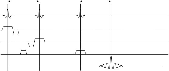
Single voxel (SV) MRS is simpler to implement. The volume of interest (VOI, or voxel) is selected using one of the two alternative data acquisition pulse sequences. The first one uses a phenomenon known as a stimulated echo to produce a signal used to generate the spectroscopic FID that is then transformed into the NMR spectrum. To produce a stimulated echo, three RF pulses are used, each rotating (flipping) the magnetization by 908. The theory of this process is too complex to be discussed in detail here; an interested reader is referred to the original paper by Hahn
(6) or to more specific texts on NMR theory, such as those listed in the Reading List section. The application of the stimulated echo method for in vivo MRS was first proposed by Frahm et al. (7) who coined an acronym STEAM (Stimulated Echo Acquisition Mode) to describe it. A simplified diagram of the stimulated echo MRS acquisition pulse sequence is shown in Fig. 8. The three RF pulses are shown on the first line of the diagram, the echo signal from the localized voxel can be seen on the bottom line of the diagram. How does this sequence allow the selection of a specific VOI as a source of collected signal? The key to successful VOI localization is to use a slice-selective RF excitation. This technology is taken straight from mainstream MRI, and thus the reader is referred to MRI-specific information for further details (see the section Magnetic Resonance Imaging or MRI monographs listed in the
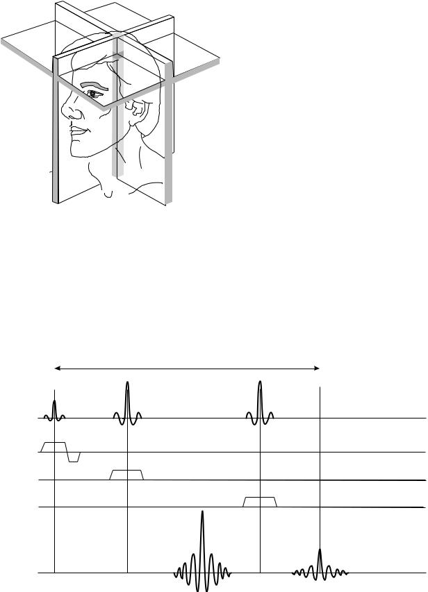
Reading List). Briefly, the slice selection technique relies on the use of band-limited RF pulses (notice the unusual modulation envelope of RF pulses shown in Fig. 8) applied in the presence of tightly controlled magnetic field gradients (MFG), shown as pulses labeled Gx, Gy, and Gz in Fig. 8. When a band-limited RF pulse is played in the presence of an MFG, only the spins in a narrow range of positions, located within a thin layer of the studied object (a slice) will achieve the resonance conditions and respond accordingly; all the spins outside the slice will be out of resonance and remain unaffected. Thus, the spin magnetization within the selected slice will be flipped by the RF, and magnetization outside the slice will remain unaffected. An analysis of this process shows that the slice orientation is perpendicular to the direction of the MFG, slice thickness is controlled by the amplitude of the MFG pulse, and location (offset from the magnet’s isocenter) is determined by the shift in carrier frequency of the RF pulse. Thus, the first pulse in Fig. 8 will excite spins in a slice that is perpendicular to the z axis of the magnet (Gz was used), the two remaining pulses will excite spins in slices perpendicular to the x and y directions, respectively. Since the condition required to produce a stimulated echo is that the spins be subject to all three pulses, only the matter located at the intersection of the three perpendicular slices fulfills the criterion, and thus only the spins located within this volume will generate the stimulated echo signals. The dimensions of the VOI selected in such a way are determined by the thickness of individual slices, and the location of the VOI is determined by the position of individual slices, as illustrated in Fig. 9.
The other single voxel MRS protocol uses a spin echo sequence to achieve volume selection. To produce the localized signal, three RF pulses are used, as before. However, while the first RF pulse still rotates the magnetization by 908, the remaining two RF pulses flip the magnetization by
TE/2 |
|
TE/2 |
|
|
|
rf
G z
G x
G y
signal
Figure 8. A simplified diagram of a basic STEAM MRS sequence. Time increases to the right, the time interval covered by this diagram is typically 100 ms. On the first line the RF pulses are shown; the next three lines show the timing of the pulses generated by the three orthogonal magnetic field gradient assemblies (one per Cartesian axis in space); the last line, labeled signal, shows the timing of the resulting stimulated echo NMR signal.
80 NUCLEAR MAGNETIC RESONANCE SPECTROSCOPY
Figure 9. The principle of VOI selection in STEAM protocol (see text for details).
1808 each. As a result, two spin echoes are produced, as shown on the bottom line of Fig. 10. The first echo contains a signal from a single column of tissue that lies at the intersection of the slices planes generated by the first and second RF pulses, while the second echo produces a signal from a single localized VOI within this column. As with the stimulated echo, the theory of this process is too complex to be discussed here; an interested reader is referred to the original paper by Hahn (6) or to more specific texts on NMR theory, such as those listed in the Reading List section.
TE
The application of dual echo spin echo method to in vivo MRS has been proposed by Bottomley (8) who coined an acronym Point Resolved Spectroscopy (PRESS) to describe it. A simplified diagram of the PRESS acquisition pulse sequence is shown in Fig. 10. The three RF pulses are shown on the first line of the diagram; but only the second echo signal seen on the bottom line of the diagram comes from the localized voxel region.
What are the advantages and weaknesses of each volume localization method? First, in both methods an echo is used to carry the spectroscopy data. Since echoes are produced by transverse magnetization, the echo amplitudes are affected by T2 relaxation and the time delay, TE, that separates the center of the echo from the center of the first RF pulse that was used to create the transverse components of magnetization. The longer the TE, the stronger the echo amplitude attenuation due to T2 effects will be. Since the amplitude of the echo signal determines the amplitude of the spectral line associated with it, the SV MRS spectra will have lines whose amplitudes will depend on the selected TE in the acquisition sequence. For the STEAM protocol, it is possible to use relatively short TE values; mostly because the magnetization contributing to the stimulated echo signal is oriented along the z axis during the period of time between the second and third RF pulses, and thus it is not subject to T2 decay (in fact, it will grow a little due to T1 relaxation recovery). Therefore, the time interval between the second and the third RF pulse is not counted toward TE. Furthermore, 908 RF pulse have shorter duration than 1808 ones, offering an additional opportunity to reduce TE. Consequently, in routine clinical applications the STEAM protocols use much shorter TE values ( 30 ms) than PRESS protocols (routine TE values used are 140 ms). Therefore, when using the
rf
G z
G x
G y
signal
Figure 10. A simplified diagram of a basic PRESS MRS sequence. Notice similarities in VOI selection algorithm within both STEAM and PRESS protocols.
STEAM protocol one is rewarded with a spectrum whose line intensities are closer to the true metabolite concentrations in the studied tissue. However, theoretical calculations show that the signal intensity of a stimulated echo is expected to be 50% less than that of a spin echo generated under identical timing conditions (i.e., TE). This is an inherent drawback of the STEAM protocol, since the spectra tend to be noticeably noisier than those produced using PRESS.
PRESS, by design, uses two spin echoes to generate a signal from localized VOI. This limits the minimum TE possible for the second echo to 80 ms or so, depending on the MR scanner hardware. Since the magnetization never leaves the transverse plane (except during RF pulses), the T2 effects are quite strong. As a result, metabolites with shorter T2 will decay down to the noise levels and vanish from the final spectrum, which has an ambivalent impact on clinical interpretations, simplifying the spectrum on one hand while removing potentially valuable information on the other. This effect can be further amplified by signal intensity oscillations with varying TE, caused by J coupling. For further details on this topic the reader is referred to the specific texts on MRS theory and applications, listed in the Reading List section.
One word of caution is called for now. The numbers quoted here reflect capabilities of MR hardware that represent a snapshot in time. As hardware improves, these parameters rapidly become obsolete.
There are other, finer arguments supporting possible preferences toward either method (STEAM or PRESS). These include such issues as suppression of parasitic signals arising from outer-volume excitation (residual signals coming from outside the VOI), sensitivity to baseline distortion of the spectra due to the use of solvent suppression, accuracy of VOI borders defined by each method, and so on. Thus, in current clinical practice there are strong propo-
NUCLEAR MAGNETIC RESONANCE SPECTROSCOPY |
81 |
nents of both STEAM and PRESS techniques, although lately PRESS seems to be gaining popularity because of simpler technical implementation issues, such as magnetic field homogeneity correction (shimming), or compensation of effects caused by eddy currents induced in the magnet cryostat by magnetic field gradient and RF pulses.
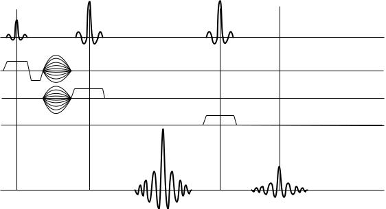
While SV MRS is relatively straightforward, and thus preferred by novices in the practice of clinical MRS, most routine applications today demand spectroscopic data collected from multiple locations within the organ studied. Therefore, a solution that would allow collection of MR spectra from multiple locations at the same time has a natural appeal to physicians. To achieve such a task is no small matter, and many schemes have been proposed before a method that today is considered most practical in daily use has been found. The method was first proposed by Brown et al. (9). Their method is both conceptually simple and revolutionary. It utilizes a method that encodes both space–(localization) and time–dependent (NMR spectra) information using mechanisms that manipulate the phases of signals emitted by individual spins at different locations. The acquisition sequence is schematically shown in Fig. 11, which illustrates the two-dimensional (2D) CSI principle using a PRESS pulse sequence. Of course, this approach is equally applicable to STEAM method as well. An astute reader will immediately recognize that the spatial encoding part of the protocol is virtually identical to dual phase encoding techniques used in 3D MRI acquisitions. At this point, readers less familiar with advanced MRI techniques probably would want to read more about this method elsewhere (see Magnetic Resonance Imaging or MRI monographs listed in the Reading List). The enlightenment occurs when one realizes that with this scheme the acquired signal is not frequency encoded at all. Therefore, after 2D FT processing in the two orthogonal spatial directions, one ends up with a collection
rf
G z
G x
G y
signal
Figure 11. A simplified diagram of a basic 2D CSI MRS sequence. The dotted gradient lobes represent phase encoding gradients responsible for multivoxel localization.
82 NUCLEAR MAGNETIC RESONANCE SPECTROSCOPY
of FIDs that are free from any residual phase errors due to spatial encoding, but nevertheless represent NMR signals from localized VOIs, anchored contiguously on a planar grid. The size and orientation of the grid is determined by the spatial encoding part of the protocol; thus, localization is conveniently decoupled from NMR frequency beats caused by the chemical shifts of studied metabolites.
If this method is so simple, why do people still want to acquire SV spectra? First, the method is quite challenging to implement successfully in practice, despite the seeming simplicity of the conceptual diagram shown in Fig. 11. Both spatial and temporal components affect the phase of collected NMR signals, and keeping them separated requires a great deal of MR sequence design wizardry and the use of advanced MR hardware. Due to peculiarities of the FT algorithm, even slight phase errors (of the order of 18) are capable of producing noticeable artifacts in the final spectra. Second, the VOI localization scheme is ill suited to a natural way of evaluating lesions spectroscopically; most clinicians like to see a spectrum from the lesion compared to a reference spectrum from a site that is morphologically equivalent, but otherwise appears normal. In the human brain, where most spectroscopic procedures are performed today, this means that the reference spectrum is acquired contralaterally to the lesion location. Such an approach represents a drawback in CSI acquisitions where VOIs are localized contiguously, and typically a few wasted voxels must be sacrificed to ensure the desired anatomic coverage of the exam. Finally, the dual-phase encoding scheme requires that each pulsed view (a single execution of the pulse sequence code with set values of both phase encoding gradients) is repeated many times to collect enough data to localize voxels correctly. As many views must be acquired as there are voxels in the grid, which causes the required number of views to grow very fast. For example, even for a modest number of locations, say 8 8, 64 views must be generated. This leads to acquisition times that appear long by today’s imaging standards (typical MRSI acquisition requires 3–8 min).
It is difficult to fully exploit the richness and diversity of technical aspects of localization techniques used in in vivo MRS; extended reviews, such as papers by Kwock (10), den Hollander et al. (11), or Decorps and Bourgeois (12), can be used as springboards for further studies.
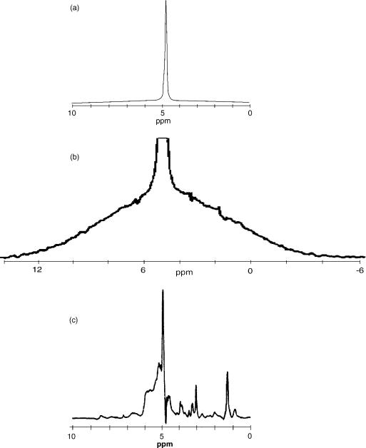
The second major challenge of in vivo 1H MRS arises from the fact that the majority of tissue matter is simply water, which for humans can vary from 28% in the bones to 99% in CSF, with an average of 75–80% in soft tissues (e.g., brain matter, muscle, lung, or liver). Thus, if a proton spectrum from just about any soft tissue (except adipose) is recorded, the result would look like the one presented in Fig. 12a, where an experimental spectrum from a muscle tissue of a young (and lean) rat, collected ex vivo on a 300 MHz NMR spectrometer, is shown. At a first glance, the result is boring: Only a single, strong peak from water is visible. Closer inspection, however, uncovers some additional details: First of all, the background of the spectrum is not totally flat, but composed of a broad peak, much wider than the normal range of chemical shifts expected in HR 1H NMR spectra. This is illustrated in Fig. 12b, where the background of the spectrum in Fig. 12a has been
enhanced by amplifying the background and cutting off most of the strong, narrow water peak. The broad spectrum is produced by protons in macromolecular components of the tissue: the proteins, DNA, RNA, and thousands of other compounds responsible for function and control of cellular activities. The spectrum broadening is caused by the residual dipolar interactions that were not fully averaged out because large molecules move more slowly than the small ones. Note: This component of the NMR signal is normally not visible in MRI and MRS applications; since the line is so broad, the relaxation time T2 of this component is quite short (on the order of hundreds of ms), thus by the time the MR signals are collected at TE that are in the range of milliseconds, this signal has decayed out. One can see some small blips on the surface of the broad line in the Fig. 12b: Those are signals from tissue biochemical compounds whose molecules are either small enough, or have specific chemical groups that are free to move relatively fast due to conformational arrangements. These clusters of protons have T2s long enough to produce narrow lines, and their chemical environment is varied enough to produce a range of chemical shifts. In short, those little blimps form an NMR spectral signature of the tissue studied. As such, they are the target of MRS. To enhance their appearance, various solvent suppression techniques are used. In solvent suppression, the goal is to suppress the strong (but usually uninteresting signal) from solvent (in case of tissue, water), thus reserving most of the dynamic range of signal recorder for small peaks whose amplitudes are close to the background of a tissue spectrum. This point is illustrated in Fig. 12c, which shows a spectrum from the same sample as the other spectra in this figure, but acquired using a water suppression technique. Now, the metabolite peaks stand out nicely against the background, in addition to some residual signal from water peak (it is practically impossible to achieve 100% peak suppression).
The most common implementation of water suppression in MRS in vivo studies uses a method known as CHESS: Chemical Shift Selective suppression, first proposed by Haase and colleagues at the annual meeting of the Society of Magnetic Resonance in Medicine in 1984. It consists of a selective 908 pulse followed by a dephasing gradient (homogeneity spoiling gradient, or homospoil). The bandwidth of the RF pulse is quite narrow, close to the width of the water line, and the carrier RF frequency offset is set to the water signal center frequency. When such a pulse is applied, only the water protons will be at resonance and they will flip by 908, leaving magnetizations of all other protons unchanged. The resultant FID from the water signal is quickly dispersed by using the homospoil gradient. When the CHESS segment is followed by a regular spectroscopy acquisition sequence (STEAM or PRESS), the first RF pulse of those spectroscopic sequences will tip all the magnetizations from metabolites, but will not create any transverse magnetization from water. The reason is that at the time the spectroscopic acquisition routine starts, the longitudinal magnetization for water protons is zero, as prepared by the CHESS routine. The description of technical details of various solvent suppression methods can be found in the paper by van Zijl and Moonen (13). The side effect of solvent suppression is a baseline distortion of the resulting spectrum;
NUCLEAR MAGNETIC RESONANCE SPECTROSCOPY |
83 |
Figure 12. An example of NMR spectra obtained from the same sample (a lean muscle from a young rat’s leg) collected in vitro: (a) standard spectrum obtained using a single RF pulse and performing an FT on the resulting FID; (b) the same spectrum scaled to reveal a wide, broad line generated by protons within macromolecules, notice small humps on top of this broad line: these are signals from small mobile macromolecules; (c) the high-resolution spectrum of the same sample, obtained using a spin–echo method and applying water suppression, both water and macromolecular peaks are suppressed, revealing small narrow lines that are subject to clinical MRS evaluations.
this distortion can be particularly severe in the vicinity of the original water peak, (i.e., at 4.75 ppm). To avoid difficulties associated with baseline correction, the MRS spectra in routine clinical applications are limited to the chemical shift range from 0 to 4.5 ppm.
In this short description of clinical MRS, the discussion had to be limited to its main features. There are many interesting details that may be of interest to a practitioner in the field, but had to be omitted here because
of space constrains; the reader is encouraged to consult comprehensive reviews, such as the work of Kreis (14), to further explore these topics.
APPLICATIONS
Now that there is a tool, it is necessary to find out what can be done with it. The clinical applications of MRS consist of
84 NUCLEAR MAGNETIC RESONANCE SPECTROSCOPY
three steps: first, an MR spectrum is acquired from the VOI; second, specific metabolite peaks are identified within the spectrum; and third, clinical information is derived from the data, mostly by assessing relative intensities of various peaks. The first step has been covered, so let us now look at step two. The easiest way to implement the spectral analysis is to create a database of reference spectra and perform either spectrum fitting or assign individual peaks by comparing the experimental data to the reference spectra. This is easier said than done; the reliable peak assignment in NMR spectra acquired in vivo has been one of the major roadblocks in the acceptance of MR spectroscopy in clinical practice.
Currently, the majority of clinical MRS studies are performed in the human brain. Over the past several years, a database of brain metabolites detectable by proton MRS in vivo has been built and verified. This process is far from finished, as metabolites with lower and lower concentrations in the brain tissue are identified by MRS and their clinical efficacy is explored. A list of components routinely investigated in current clinical practice is shown in Table 1. Even a short glance at this list immediately reveals the first major canon of the MRS method: more than a cursory knowledge of organic and biochemistry is required to fully comprehend the information available. An appreciation of the true extent of this statement can be quickly gained by taking a closer look at the first molecule listed in that table: N-acetylaspartate, or NAA. This compound belongs to a class of N-alkanoamines; the italic letter N represents the so-called locant, or a location of the secondary group attached to the primary molecule. In this case, N is a locant for a group that is attached to a nitrogen atom located within the primary molecule. The primary molecule in this case is an L-aspartic acid, which is a dicarboxylic amino acid. Dicarboxylic means that the molecule contains two carboxylic (COOH) groups. As an amino acid, L-aspartic acid belongs to the group of the so-called nonessential amino acids, which means that under normal physiological conditions sufficient amounts of it are synthesized in the body to meet the demand and no dietary ingestion is needed to maintain the normal function of the body. The N-acetyl prefix identifies a molecule as a secondary amine; in such compounds the largest chain of carbon compounds takes the root name (aspartic acid), and the other chain (the acetyl group, CH3CO–, formed by removal of the OH group from the acetic acid CH3COOH) becomes a substituent, whose location in the chain (the N-locant) identifies it as attached to the nitrogen atom. But what about the L prefix in the L-aspartic acid mentioned above? It has to do with a spatial symmetry of the molecule’s configuration. The second carbon in the aspartic chain has four bonds (two links to other carbon atoms, one link to the nitrogen atom, and the final link to a proton). These four bonds are arranged in space to form a tetrahedron with the four atoms just mentioned located at its apexes. Such a configuration is called a chiral center, to indicate a location where symmetry of atom arrangement needs to be documented. There are two ways to distribute four different atoms among four corners of a tetrahedron, one is called levorotatory (and abbreviated by a prefix L-), and the other is called dextrorotatory (and abbreviated by a prefix D-). It
turns out that the chirality of the molecular configuration has a major significance in biological applications: Since successful mating of different molecules requires that their bonding sites match, only one chiral moiety is biologically active. In our case, L-aspartic acid is biologically active; the D-aspartic acid is not. Last, but not least, the reader has probably noticed that the name of the molecule is listed as N-acetylaspartate, while we keep talking about aspartic acid. . . well, when an acid is dissolved in water, it undergoes dissociation into anions and cations; the molecule of aspartic acid in the water solution looses two protons from the carboxylic groups COOH (the locations of the cleavages are indicated by asterisks in the structural formulas shown in Table 1), and becomes a negatively charged anion. To reflect this effect, and suffix - ate is used. Thus, the name N-acetylaspartate describes an anion form of a secondary amine, whose primary chain is a levorotatory chiral form of aspartic group, with a secondary acetyl group attached to the nitrogen atom. The NAA is so esoteric a molecule that most standard biochemistry books do not mention it at all; its chief claim to prominence comes from the fact that it is detectable by MRS. A recent review of NAA metabolism has been recently published by Barlow (15).
The example discussed above emphasizes that much can be learned just from a name of a biological compound. To gain more literacy in the art of decoding the chemical nomenclature of biologically active compounds, the reader is encouraged to consult the appropriate resources, of which the Introduction to Subject index of CAS (16) is one of the best.
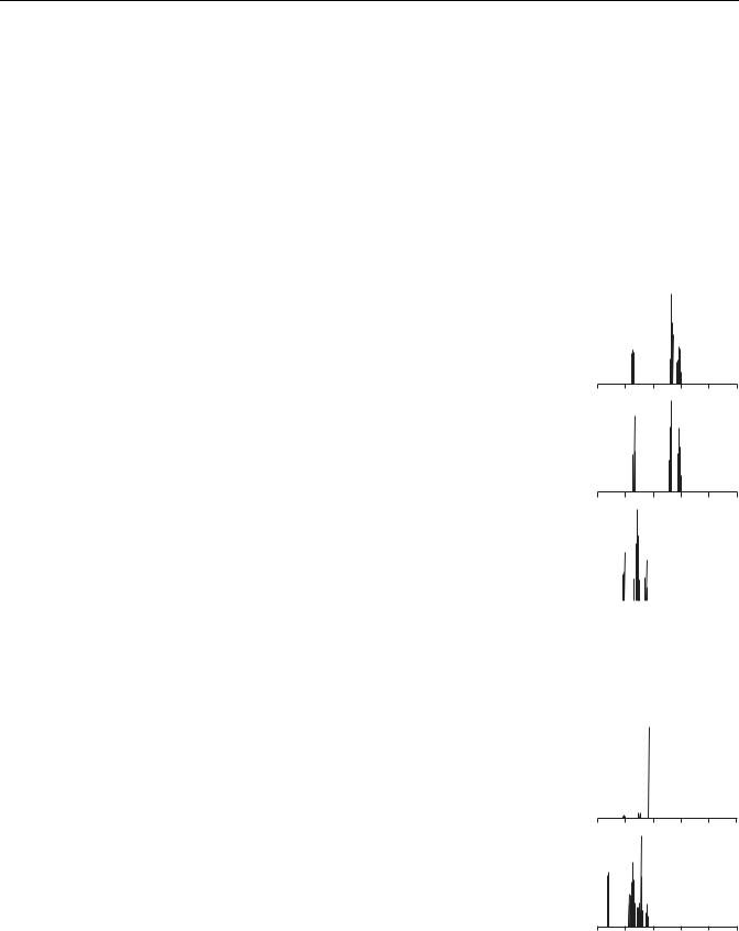
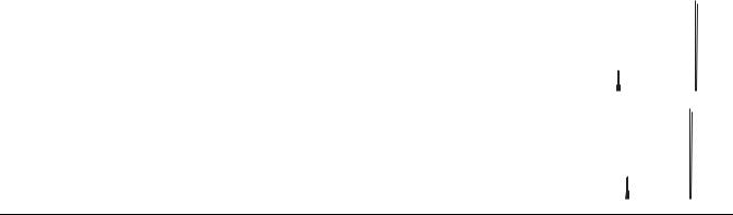
As mentioned earlier, routine clinical MRS studies focus on proton spectra spanning the range from 0 to 4.5 ppm; the NMR properties of compounds listed in Table 1 are presented in Table 2, which identifies each molecular group according to carbon labeling used in structural formulas shown in Table 1. For each molecular group, the chemical shift of the main NMR peak is listed, along with the spectral multiplet structure characterizing this line. A simulated theoretical spectrum shows all lines in the range from 0 to 5 ppm, to give the reader an idea where the molecular signature peaks are located in the spectra acquired in vivo. Finally, information is provided whether, for a particular line, the signal acquired in standard MRS in vivo studies is strong enough to emerge above the noise levels and become identifiable. This information is further supplemented with comments indicating whether a particular line is expected to be visible on spectra acquired with short or long TE values. It is evident that the information provided in Table 2 is absolutely critical to successful interpretation of clinical MRS results; unfortunately, space limitations prevent us from further dwelling into details of spectral characteristics of clinically important metabolites. This information can also be difficult to locate in the literature since most of the data still reside in original research papers; fortunately, a recent review by Govindaraju et al. (17) offers an excellent starting point.
An examination of data shown in Table 2 quickly leads to a realization that only a limited number of metabolite signature lines can be successfully used in the
|
|
|
|
NUCLEAR MAGNETIC RESONANCE SPECTROSCOPY |
85 |
|||||||||
Table 1. Basic Properties of Metabolites Most Commonly Detected in MRS Spectra of the Human Brain |
|
|
||||||||||||
|
|
|
|
|
|
|
|
|
|
|
|
|
|
|
|
|
|
|
|
|
|
|
|
|
|
|
|
Normal |
|
|
|
|
|
|
|
|
|
|
|
|
|
|
Concen- |
|
|
|
|
|
|
|
|
|
|
|
|
|
|
tration |
|
|
|
|
|
|
|
|
|
|
|
|
|
|
Range in |
|
|
|
|
|
CASa |
|
|
|
|
|
|
Molecular |
brain, |
|
|
Metabolite |
Full Name |
Acronym |
Formula |
Number |
Structure |
Weight |
mmol |
|
||||||
|
|
|
|
|
|
|
|
|
|
|
|
|
|
|
N-Acetylaspartate N-Acetyl-L-aspartic |
NAA |
C6H9NO5 |
[997-55-7] |
|
|
|
|
COO*H |
175.14 |
8–17 |
|
|||
|
acid; amino acid |
|
|
CH3 |
|
|
NH |
|
|
|
|
|
|
|
|
|
|
CO |
|
|
|
CH |
|
|
|
||||
|
|
|
|
|
|
|
|
|
|
|||||
|
|
|
|
|
|
|
|
|
|
|
|
|
|
|
|
|
|
|
|
|
|
CH2 |
|
|
|
||||
|
|
|
|
|
NH |
|
|
|
|
|
|
|
|
|
|
|
|
|
|
COO*H |
|
|
|
||||||
Creatine |
(1-Methylguanidino) |
Cr |
C4H9N3O2 |
[57-00-1] |
|
acetic acid; |
|
|
|
|
non-protein |
|
|
|
|
amino acid |
|
|
|
Glutamate |
L-Glutamic acid; |
Glu |
C5H9NO4 |
[56-86-0] |
|
amino acid |
|
|
|
Glutamine |
L-Glutamic |
Gln |
C5H10N2O3 |
[56-85-9] |
|
acid-5-amide; |
|
|
|
|
amino acid |
|
|
|
myo-Inositol |
1,2,3,5/4,6- |
m-Ins |
C6H12O6 |
[87-89-8] |
|
Hexahydroxy- |
|
|
|
|
cyclohexane |
|
|
|
Phosphocreatine |
Creatine phosphate |
PCr |
C4H10N3O5P [67-07-2] |
|
Choline |
Choline hydroxide, |
Cho |
C5H14NO |
[62-49-7] |
|
Choline base, |
|
|
|
|
2-Hydroxy- |
|
|
|
|
N,N,N-trimethyl- |
|
|
|
|
athanaminium |
|
|
|
Glucose |
D-Glucose, dextrose |
Glc |
C6H12O6 |
[50-99-7] |
|
anhydrous, corn |
|
|
|
|
sugar, grape sugar |
|
|
|
Lactate |
L-Lactic acid, |
Lac |
C3H6O |
[79-33-4] |
|
2-hydroxypropanoic |
|
|
|
|
acid |
|
|
|
Alanine |
L-Alanine, 2-amino- |
Ala |
C3H7NO2 |
[65-41-1] |
|
propanoic acid |
|
|
|
NH2 C N CH2 COO*H
CH3
COO*H
`NH2 CH
CH2
CH2
COO*H
COO*H
`NH2 CH
CH2
CH2
CO
NH2
OH
OH OH
OH OH 
OH
O NH
H*O P NH C N CH2 COO*H
O*H CH3
OH
CH2
CH2
CH3 N CH3
CH3
CH2OH
O
OH
OH |
OH |
OH
COO*H
OH CH
CH3
COO*H
`NH2 CH
CH3
131.145–11
147.136–13
146.153–6
180.24–8
211.113–6
104.200.9–2.5
180.151.0
90.070.4
89.090.2–1.4
aCAS ¼ Chemical Abstracts Service Registry Number of the neat, nondissociated compound. In structural formulas, an asterisk indicates a site where, upon dissociation, a proton is released; apostrophe` indicates a site where, upon dissociation, a proton is attached. Metabolite names refer to dissociated (ionic) forms of the substances since this is the form they are present in the in vivo environment.
86 NUCLEAR MAGNETIC RESONANCE SPECTROSCOPY
Table 2. The NMR Properties of Metabolites Most Commonly Detected in MRS Spectra of the Human Brain
|
|
|
|
|
|
Theoretical |
|
|
|
|
|
|
|
|
|
|
|
|
|||||||||
|
|
Molecular |
Chemical |
Multiplet |
Visibility |
Spectrum –Range |
|
|
|
|
|
||||||||||||||||
Metabolite |
Acronym |
|
Group |
Shift d ppma |
Structureb |
in vivoc |
(0,5) ppm |
|
|
|
|
|
|
|
|
|
|
|
|
||||||||
|
|
|
|
|
|
|
|
|
|
|
|
|
|
|
|
|
|
|
|
|
|
|
|
|
|
|
|
N-Acetylaspartate |
NAA |
CH3 |
Acetyl |
2.00 |
s |
Yes |
|
|
|
|
|
|
|
|
|
|
|
|
|
|
|
|
|
|
|
||
|
|
|
|
|
|
|
|
|
|
|
|
|
|
|
|
|
|
|
|||||||||
|
|
CH2 |
Aspartate |
2.49 |
dd |
No |
|
|
|
|
|
|
|
|
|
|
|
|
|
|
|
|
|
|
|
||
|
|
CH2 |
Aspartate |
2.67 |
dd |
No |
|
|
|
|
|
|
|
|
|
|
|
|
|
|
|
|
|
|
|
||
|
|
CH Aspartate |
4.38 |
dd |
No |
|
|
|
|
|
|
|
|
|
|
|
|
|
|
|
|
|
|
|
|||
|
|
|
|
|
|
|
|
|
|
|
|
|
|
|
|
|
|
|
|
|
|
|
|
|
|
|
|
|
|
|
|
|
|
5 |
4 |
3 |
2 |
1 |
0 |
||||||||||||||||
Creatine |
Cr |
N-CH3 |
3.03 |
s |
Yes |
|
|
|
|
|
|
|
|
|
|
|
|
|
|
|
|
|
|
|
|||
|
|
|
|
|
|
|
|
|
|
|
|
|
|
|
|
|
|
|
|||||||||
|
|
CH2 |
|
3.91 |
s |
Yes |
|
|
|
|
|
|
|
|
|
|
|
|
|
|
|
|
|
|
|
||
|
|
|
|
|
|
|
|
|
|
|
|
|
|
|
|
|
|
|
|
|
|
|
|
|
|
|
|
5 |
4 |
3 |
2 |
1 |
0 |
Glutamate |
Glu |
CH2 |
2.07 |
m |
Yes, on short TE |
|
|
CH2 |
2.34 |
m |
Yes, on short TE |
|
|
CH |
3.74 |
dd |
No |
5 |
4 |
3 |
2 |
1 |
0 |
Glutamine |
Gln |
CH2 |
2.12 |
m |
Yes |
|
|
CH2 |
2.44 |
m |
Yes |
|
|
CH |
3.75 |
t |
No |
|
|
CH |
|
|
5 |
4 |
3 |
2 |
1 |
0 |
|||||
Myo-inositol |
m-Ins |
3.27 |
t |
No |
|
|
|
|
|
|
|
|
|
||
|
|
CH, CH |
3.52 |
dd |
Yes, on short TE |
|
|
|
|
|
|
|
|
|
|
|
|
CH, CH |
3.61 |
t |
Yes, on short TE |
|
|
|
|
|
|
|
|
|
|
|
|
CH |
4.05 |
t |
No |
|
|
|
|
|
|
|
|
|
|
|
|
|
|
|
|
|
|
|
|
|
|
|
|
|
|
|
|
|
|
|
5 |
4 |
3 |
2 |
1 |
0 |
|||||
Phosphocreatine |
PCr |
N-CH3 |
3.03 |
s |
Yes |
|
|
|
|
|
|
|
|
|
|
|
|
|
|
|
|
|
|
|
|||||||
|
|
CH2 |
3.93 |
s |
Yes |
|
|
|
|
|
|
|
|
|
|
|
|
|
|
|
|
|
|
|
|
|
|
|
|
|
|
5 |
4 |
3 |
2 |
1 |
0 |
Choline |
Cho |
N-(CH3)3 |
3.18 |
s |
Yes |
|
|
CH2 |
3.50 |
m |
No |
|
|
CH2 |
4.05 |
m |
No |
5 |
4 |
3 |
2 |
1 |
0 |
Glucose |
Glc |
b– CH |
4.63 |
d |
Not visible in |
|
|
|
|
|
normal brain |
|
|
All other CH |
3.23–3.88 |
m |
due to low |
|
|
|
|
|
concetration |
5 |
4 |
3 |
2 |
1 |
0 |
|
|
|
|
NUCLEAR MAGNETIC RESONANCE SPECTROSCOPY |
|
|
87 |
||||||||||
Table 2. (Continued) |
|
|
|
|
|
|
|
|
|
|
|
|
|
|
|
|
|
|
|
|
|
|
|
|
|
|
|
|
|
|
|
||||
|
|
|
|
|
|
|
|
|
Theoretical |
|
|
|
|
||||
|
|
Molecular |
Chemical |
Multiplet |
Visibility |
|
|
Spectrum –Range |
|||||||||
Metabolite |
Acronym |
Group |
Shift d ppm |
Structure |
in vivo |
|
|
(0,5) ppm |
|
|
|
|
|||||
Lactate |
Lac |
CH3 |
1.31 |
d |
Not visible in |
|
|
|
|
|
|
|
|
|
|
|
|
|
|
CH |
|
|
normal brain |
|
|
|
|
|
|
|
|
|
|
|
|
|
|
4.10 |
q |
due to low |
|
|
|
|
|
|
|
|
|
|
|
||
|
|
|
|
|
concetration |
|
|
|
|
|
|
|
|
|
|
|
|
|
|
|
|
|
|
|
|
|
|
|
|
|
|
|
|
|
|
|
|
CH3 |
|
|
5 |
4 |
3 |
2 |
1 |
0 |
|||||||
Alanine |
Ala |
1.47 |
d |
Not visible in |
|
|
|
|
|
|
|
|
|
|
|
||
|
|
CH |
|
|
normal brain |
|
|
|
|
|
|
|
|
|
|
|
|
|
|
3.77 |
q |
due to low |
|
|
|
|
|
|
|
|
|
|
|
||
|
|
|
|
|
concetration |
|
|
|
|
|
|
|
|
|
|
|
|
|
|
|
|
|
|
|
|
|
|
|
|
|
|
|
|
|
|
|
|
|
|
|
|
|
|
|
|
|
|
|
|
|
|
|
|
|
|
|
|
|
5 |
4 |
3 |
2 |
1 |
0 |
|||||||
aThe bold type indicates a dominant line in the spectrum.
bs ¼ singlet, d ¼ doublet, dd ¼ doublet of doublets, t ¼ triplet, q ¼ quadruplet, m ¼ multiplet.
cReference to short TE indicates that those signals have short T2s and thus will be suppressed in acquisitions with long TE.
interpretation of clinical proton MRS spectra. In normal volunteers, five major markers can routinely be detected and evaluated:
The N-acetylaspartate peak at 2.0 ppm, commonly referred to as NAA.
The combination of creatine (Cr) and phosphocreatine (PCr); reported together as two lines positioned 3.0 and 3.9 ppm, respectively. Mostly referred to as Cr, but some people use a label tCr (for total creatine). The peak at 3.0 ppm is often identified as Cr, and the peak at 3.9 ppm as Cr2,
The combination of glutamine (Gln) and glutamate (Glu) at 2.2–2.4 ppm; since the peaks from those two compounds strongly overlap and are typically unresolvable, the are routinely reported together and referred to as Glx.
The choline peak at 3.25 ppm, referred to as Cho; The primary contributions to this peak are from bound forms of choline: phosphorylcholine (PC) and glycerophosphorylcholine (GPC), with only minor signal from free choline.
The myo-inositol group at 3.6 ppm is visible only in spectra acquired with short TE (due to J coupling effects that suppress the intensity of lines forming this signal at long TEs). Myo-inositol name poses evidently a challenge to acronym creators, since it can be found labeled as m-Ins, MI, mI, and In.
In addition, the following markers are routinely evaluated in a variety of diseases:
Lactate (Lac), often visible as a doublet at 1.3 ppm. Mobile lipds (Lip) whose methyl (CH3) groups are visible
at 0.9 ppm and methylene (CH2) groups provide signal at 1.3 ppm.
In special cases other metabolites may become visible, and we list here two examples:
Alanine (Ala) with a signature peak at 1.5 ppm. Glucose (Glc), mostly showing as a broad peak 3.5 ppm;
note that the theoretical spectrum shown in Table 2 is a superposition of a- and b-anomers that occur in 1:2 ratio, respectively, in equilibrium in vivo conditions.
Examples of typical MRS spectra obtained from healthy subjects are shown in Fig. 13. The first thing to notice is that the signal noise ratio in those spectra is poor, so indeed, only the strongest lines from metabolites listed in Table 2 have a chance to become visible.
In the context of this discussion, the following questions have been discussed: What is MRS, how to perform it, who is interested in those studies, and why? If an actual clinical MRS examination were being performed, at this stage of MRS study we would have localized the lesion, collected an in vivo MR spectrum from the tissue within this lesion, identified the signature metabolite peaks, and analyzed their relative intensities. Now would have come the time to ponder what the results mean and what is their clinical significance. It is not an easy task, since the last analytic step listed above produces results that must be compared to ‘‘normal’’ baseline references. These reference data are obtained by performing statistical analysis of multiple results obtained from healthy people: a challenging task given biological diversity of normal subjects. Thus, MRS results are reported using such imprecise terms as unchanged, elevated, or suppressed. Sometimes, when clinicians want to be particularly precise, they will report ratios, such as the NAA/Cr ratio, which essentially renormalizes all observed signal intensities by assigning an arbitrary intensity of one unit to the Cr peak. In other words, this approach uses the Cr peak as an internal reference. As mentioned in Table 3, the rationale for such
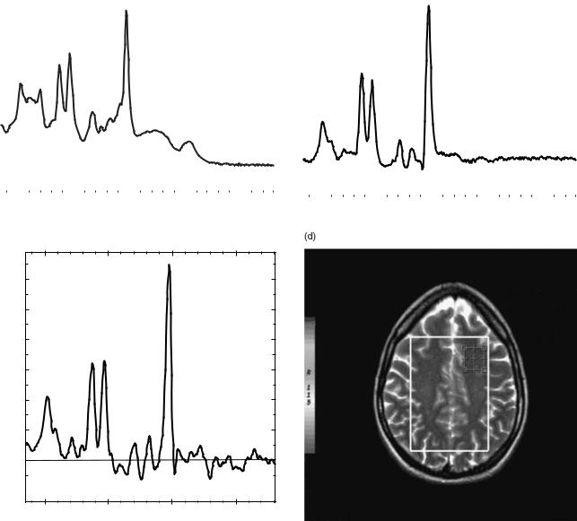
88 |
NUCLEAR MAGNETIC RESONANCE SPECTROSCOPY |
|
|
(a) |
NAA |
NAA |
|
(b) |
|||
|
|
||
|
Cr |
|
|
|
Cho |
Cho |
Cr2 |
Cr |
|
mL |
||
|
||
|
Glx |
|
|
Cr2 |
Glx
|
|
|
|
|
|
|
|
|
|
|
|
|
|
|
|
|
|
|
|
|
|
|
|
|
|
4 |
3 |
2 |
1 |
0 |
|
4 |
3 |
2 |
1 |
0 |
|||||||||||||||
|
|
|
|
|
|
|
|
|
|
|
|||||||||||||||
(c)
NAA
1200
1000
800
Cr
Cho
600
Cr2
400
200 |
Glx |
0
4 |
3 |
2 |
1 |
Figure 13. Examples of typical MRS spectra obtained in vivo for a normal volunteer: (a) STEAM SV protocol with TE ¼ 30 ms and TR of 2000 ms, magnitude mode; (b) PRESS SV protocol with TE ¼ 144 ms and TR ¼ 1500 ms, magnitude mode; (c) PRESS 2D CSI with TE ¼ 135 ms, TR ¼ 1000 ms, 16 16 voxel locations, real mode; (d) Image reference showing a location of selected VOI associated with the spectrum shown in (c) The VOI is generated by combining voxel locations. All data acquired within a single study, lasting 15 min; spectra (a) and (b) were acquired at the same location using the same VOI size, no signal averaging was used (NEX ¼ 8).
an approach is that the levels of Cr tend to be relatively stable under normal physiologic conditions. Such findings are purely phenomenological and their value is established over time by practicing evidence-based medicine, that is by performing statistical analysis of a large number of findings and looking for correlations between MRS results and the patient’s clinical status. The drawback of such an approach is that in the early stages of new methodology, there is no established consensus regarding data interpretation, thus one is forced to read a large number of published clinical reports and develop one’s
own approach to the inclusion of MRS findings into the clinical decision making process. A short summary of the current understanding of clinical findings related to MRS results is provided in Table 3. However, since these findings are still subject to frequent updates, it would have been pointless to try to provide in-depth coverage of these issues here, knowing full well that the data are likely to be obsolete by the time this publication appears in print. Instead, the reader is strongly encouraged to survey the current literature for reviews of clinical MRS topics; some excellent, previously published papers can serve as a
|
|
|
NUCLEAR MAGNETIC RESONANCE SPECTROSCOPY |
89 |
||
Table 3. Clinical Properties of Metabolites Most Commonly Detected in MRS Spectra of the Human Brain |
|
|
||||
|
|
|
|
|
|
|
Metabolite |
Full Name |
Acronym |
Function |
Pathological Variation |
|
|
|
|
|
|
|
|
|
N-Acetylas- |
N-Acetyl-L- |
NAA |
Plays osmoregulatory function |
Decrease in NAA levels is indicative of reversible |
|
|
partate |
aspartic acid; |
|
in the intercompartmental |
axonal injury or neuronal loss. In adults it has |
|
|
|
amino acid |
|
system, thought to be |
been associated with neoplasia, multiple sclerosis, |
||
|
|
|
responsible for the removal |
hypoxia, ischemia, stroke, trauma, epilepsy, |
|
|
|
|
|
of intracellular water, against |
encephalitis, and neurodegenerative syndromes |
|
|
|
|
|
the water gradient, from |
|
|
|
|
|
|
myelinated neurons |
|
|
|
Creatine |
(1-Methylgu- |
Cr |
Synthesized in the liver, it is |
Levels of creatine and phosphocreatine are tightly |
|
|
|
anidino)acetic |
|
exported to muscle and brain |
controlled under physiologic conditions, and thus |
|
|
|
acid |
|
where it is phosphorylated into |
this peak has been suggested as an internal |
|
|
|
|
|
phosphocreatine and used as |
reference for metabolite amplitude or area ratios. |
|
|
|
|
|
an energy store |
Increased levels of Cr and PCr have been observed, |
||
|
|
|
|
however, in hyperosmolar states, as well as |
|
|
|
|
|
|
in trauma. They also increase with aging |
|
|
Glutamate |
L-Glutamic acid; |
Glu |
Most abundant amino acid found |
Plays a role in detoxification of ammonia in the |
|
|
|
amino acid |
|
in the human brain, acts as an |
hyper ammonemic states |
|
|
|
|
|
excitatory neurotransmitter |
|
|
|
Glutamine |
L-Glutamic |
Gln |
Plays a role in glutamate |
Elevated levels of glutamate and glutamine have |
|
|
|
acid-5-amide; |
|
regulation; astrocytes metabolize |
been observed in hepatic encephalopathy, |
|
|
|
amino acid |
|
glutamate to glutamine, thus |
Reyes syndrome, meningiomas, and rare inherited |
||
|
|
|
preventing excitotoxicity |
enzyme deficiency. Reduced levels have been |
|
|
|
|
|
|
associated with Alzheimer’s disease |
|
|
myo- |
1,2,3,5/4,6- |
m-Ins |
A component of |
Concentration fluctuates more than that of any other |
||
Inositol |
Hexahydroxy- |
|
membrane phospholipids, |
major metabolite in the brain. Increased levels of |
|
|
|
cyclo hexane |
|
functions as a cerebral osmolyte. |
myo-inositol have been observed in neonates, |
|
|
|
|
|
It is also thought to play |
Alzheimer’s disease, diabetes, and hypersomolar |
|
|
|
|
|
an essential role in cell growth |
states. myo-Inositol levels are decreased in |
|
|
|
|
|
|
hepatic encephalopathy, hypoxia, stroke, and some |
||
|
|
|
|
neoplasms |
|
|
Phospho- |
Creatine |
PCr |
A major energy storage in the body |
See notes for creatine. |
|
|
creatine |
phosphate |
|
|
|
|
|
Choline |
Choline hydroxide, Cho |
Choline is important for normal |
Increased levels of choline have been detected in |
|
|
|
|
Choline base, |
|
cellular membrane composition |
normal infants, and aging adults. They were also |
|
|
|
2-Hydroxy-N,N, |
|
and repair, normal brain function |
associated with neoplasia, gliosis, demyelinating |
|
|
|
N-trimethyl- |
|
and normal cardiovascular function |
disease, inflammation or infection, trauma, |
|
|
|
athanaminium |
|
|
diabetes, chronic hypoxia, and AIDS. |
|
|
|
|
|
|
Decreased levels of choline |
|
|
|
|
|
|
have been found in hepatic encephalopathy, stroke, |
||
|
|
|
|
and dementias, including Alzheimer’s disease |
|
|
Glucose |
D-Glucose |
GLc |
A major energy carrier |
Increased levels notes in diabetes mellitus, parental |
||
|
|
|
throughout the body. |
feeding, hypoxic encephalopathy |
|
|
Lactate |
L-Lactic acid, |
Lac |
Lactate is a signature byproduct |
Visible in a variety of diseases. Increased levels of |
|
|
|
2-hydroxypro- |
|
of carbohydrate catabolism and |
lactate were observed in some tumors, during |
|
|
|
panoicacid |
|
thus when normal cellular |
the first 24 h after infarction, in hypoxia, anoxia, |
|
|
|
|
|
oxidative respiration mechanisms |
near-drowning, and hypoventilation |
|
|
|
|
|
are active, its levels in the brain |
|
|
|
|
|
|
tissues are very low |
|
|
|
Alanine |
L-Alanine, |
ALa |
Alanine is a nonessential amino |
The alanine peak is difficult to detect since it is easily |
||
|
2-Aminopro- |
|
acid of uncertain function |
overshadowed by lactate. Alanine |
|
|
|
panoic acid |
|
in the brain |
levels might be elevated in meningiomas |
|
|
Lipids |
Fatty acids, |
Lip |
Normally the lipid signals are not |
Mobile protons from lipids (0.9 ppm for CH3 and |
|
|
|
glycerides, |
|
visible in the MRS spectra of the |
1.3 ppm for CH2) are not normally visible in |
|
|
|
glycolipids, |
|
brain, but might appear |
brain spectra, but can appear in diseased conditions. |
||
|
lipoproteins |
|
due to fat contamination |
Lipid signals are suppressed at long TEs. Elevated |
||
|
|
|
(voxel bleed) |
lipid levels are observed in cellular necrosis, |
|
|
|
|
|
|
high-grade astrocytoma, and lymphoma |
|
|
|
|
|
|
|
|
|
starting point (18–21). The last paper on this list, by Smith and Stewart (21), also offers excellent overview of spectroscopy studies in organs other than the brain.
It is impossible, in one short article, to offer a fully comprehensive coverage of such an advanced and rapidly
evolving discipline as clinical magnetic resonance spectroscopy. The author can only hope that this brief overview offers sufficient information and enough reference pointers to let the readers start exploring this new and exciting field on their own.