Fractionation: the linear-quadratic approach

8.1 INTRODUCTION

Major developments in radiotherapy fractionation have taken place during the past three decades and these have grown out of understanding in radiation biology. The relationships between total dose and dose per fraction for lateresponding tissues, acutely responding tissues and tumours provide the basic information required to optimize radiotherapy according to the dose per fraction and number of fractions.

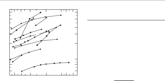
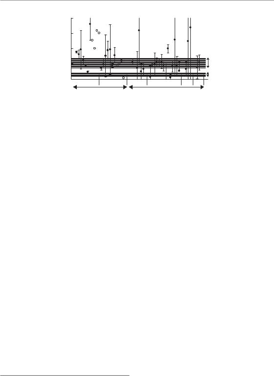
A milestone in this subject was the publication by Thames et al. (1982) of a survey of isoeffect curves for various normal tissues, mainly in mice. Their summary is shown in Fig. 8.1. Each of the investigations contributing to this chart was a study of the response of a normal tissue to fractionated radiation treatment using a range of doses per fraction. In order to minimize the effects of repopulation, the survey was restricted to studies in which the overall time was kept short by the

use of multiple treatments per day, or ‘where an effect of regeneration of target cells was shown to be unlikely’. This summary thus represents the influence of dose per fraction on response and mostly excludes the influence of overall treatment time. It was possible in each study, and for each chosen dose per fraction, to determine the total radiation dose that produced some defined level of damage to the normal tissue. These endpoints of tolerance differed from one normal tissue or experimental study to another. Each line in Fig. 8.1 is an isoeffect curve determined in this way. The dashed lines show isoeffect curves for acutely responding tissues and the full lines are for lateresponding tissues. Note that fraction number increases from left to right along the abscissa and therefore the dose per fraction scale decreases from left to right. The results of this survey show that the isoeffective total dose increases more rapidly with decreasing dose per fraction for late effects than for acute effects. If the vertical axis is

Dose/fraction (Gy)

Figure 8.1 Relationship between total dose and dose per fraction for a variety of normal tissues in experimental animals. The results for late-responding tissues (unbroken lines) are systematically steeper than those for early-responding tissues (broken lines). From Thames et al. (1982), with permission.

regarded as a tissue tolerance dose, it can be deduced immediately from this plot that using lower doses per fraction (towards the right-hand end of the abscissa) will tend to spare late reactions if the total dose is adjusted to keep the acute reactions constant.

The linear-quadratic (LQ) cell survival model, introduced in Chapter 4, can be used to describe this relationship between total isoeffective dose and the dose per fraction in fractionated radiotherapy. The LQ model can thus form a robust quantitative environment for considering the balance between acute and late reactions (and effect on the tumour) as dose per fraction and total dose are changed. This is one of the most important developments in radiobiology applied to therapy. In this chapter, we present the theoretical background and supporting data that have led to the wide adoption of the LQ approach to describing fractionation and we show the basic framework from which calculations can be made using this model. Examples of such calculations in a clinical setting are demonstrated practically in Chapter 9.

8.2 HISTORICAL BACKGROUND: LQ VERSUS POWER-LAW MODELS

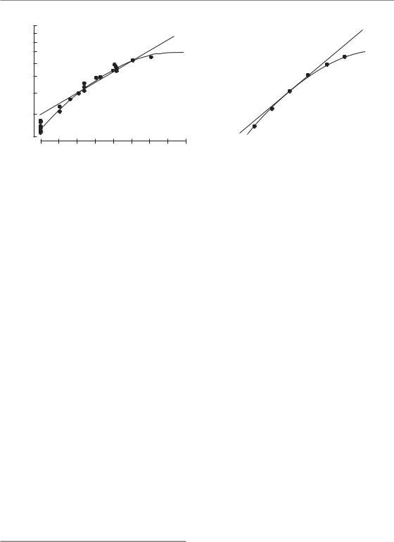
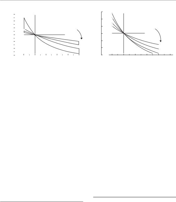
Two specific examples of isoeffect plots for radiation damage to normal tissues in the mouse are shown in Fig. 8.2: skin is an early-responding tissue and kidney a late-responding tissue. In each case the total radiation dose to give a fixed level of damage is plotted against dose per fraction and fraction number on a double log plot. Note that the curve for kidney is steeper than that for skin.

The solid lines in Fig. 8.2 are calculated by an equation based on the LQ model:

where d is the dose per fraction (see Section 8.4 for for the derivation of this equation). The steepness and curvature of these lines are both determined by one parameter: the / ratio. For the skin data (Fig. 8.2a), the / ratio is about 10. The units of / are grays, so the / ratio in this case is 10 Gy. For the kidney data / is about 3 Gy.

The LQ model fits these data very well and produces curves in this type of log–log plot. Also shown in Fig. 8.2 are broken lines showing the fit of Ellis’ ‘Nominal Standard Dose’ (NSD) model (Ellis, 1969) to both datasets. This is an example of a simple power-law relationship between total dose and number of fractions, and it and its derivatives such as TDF (time–dose–fractionation) were in clinical use for many years. The equation for NSD is:

Total dose NSD N0.24 T 0.11

In these animal studies the overall treatment time (T) was constant. Power-law models such as NSD and TDF give straight lines in this type of plot and fit the skin data well from 4 to 32 fractions, but the data points fall below the broken line for both small and large doses per fraction. The discrepancy for doses per fraction of 1–2 Gy is important in relation to hyperfractionation (see Section 8.6). For late reactions, as illustrated by the kidney data in Fig. 8.2b, the NSD formula again does not fit as well as the LQ formula, even though the N exponent has been raised from 0.24 to 0.35 in order to

Total dose (Gy)

(a)

allow for the greater slope. A similar modification, but not necessarily by the same amount, must be made for all late-responding tissues if the NSD formulation is to be even approximately correct.

A crucial therapeutic conclusion is illustrated by these two sets of data. At both ends of the scale, in the region of large and small dose per fraction, power-law equations overestimate the actual tolerance dose (as shown by the experimental and clinical data). This means that the power-law models are unsafe in these regions, a conclusion that is well supported by clinical experience. At the present time it is strongly recommended that the LQ model should always be used, with a correctly chosen α/β ratio, to describe isoeffect dose relationships at least over the range of doses per fraction between 1 and 5 Gy. The LQ model is simple to use in clinical calculations and comparisons, and does not require the use of ‘look-up tables’. Sections 8.4–8.8 and Chapter 9 provide a straightforward guide to LQ calculations.

8.3 CELL-SURVIVAL BASIS OF THE LQ MODEL

What is the explanation for the difference between the fractionation response of earlyand

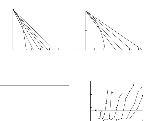
late-responding tissues which is shown in Figs 8.1 and 8.2? Figure 8.3 shows hypothetical single-dose (one-fraction) survival curves for the target cells in earlyand late-responding tissues, drawn according to the LQ equation (see Chapter 4, Fig. 4.5b). E represents the reduction in cell survival (on a logarithmic scale) that is equivalent to tissue tolerance. The total dose that would need to be given in two fractions is obtained by drawing a straight line from the origin through the survival curve at E/2 and measuring the intersection of this line with the dose axis. As shown by the dashed line labelled 2 in Fig. 8.3a, a dose of around 11 Gy takes the effect down to E/2 and (with assumed constant effect per fraction) a second 11 Gy gives the isoeffect E: the total isoeffect dose is approximately 22 Gy. This compares with a single dose of approximately 14 Gy to give the same isoeffect E, shown by the solid line. The total dose for three fractions is obtained in the same way by drawing a line through E/3 on the survival curve, and similarly for the other fraction numbers. Because the late-responding survival curve (Fig. 8.3b) is more ‘bendy’ (it has a lower α/β ratio), the isoeffective total dose increases more rapidly with increasing number of fractions than the earlyresponding tissue in which the survival curve bends less sharply.

Log (surviving fraction)

(a)

8.4 THE LQ MODEL IN DETAIL

The surviving fraction (SFd) of target cells after a dose per fraction d is given in Chapter 4, Section 4.10, as:

SFd exp( αd βd2)

Radiobiological studies have shown that each successive fraction in a multidose schedule is equally effective, so the effect (E) of n fractions can be expressed as:

Eloge(SFd)n n loge(SFd)

n(αd βd2)

αD βdD

where the total radiation dose D nd. This equation may be rearranged into the following forms:

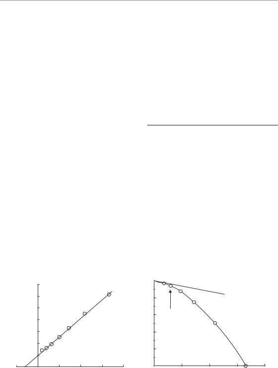
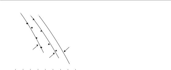
The practical working of these equations may be illustrated by the results of careful fractionation experiments on the mouse kidney (Stewart et al., 1984). In these experiments, functional damage to the kidneys was measured by ethylenediaminetetraacetic acid (EDTA) clearance up to 48 weeks after irradiation with 1–64 fractions. Figure 8.4 shows the response measured as a function of total

Figure 8.4 Dose–response curves for late damage to the mouse kidney with fractionated radiation exposure. Damage is indicated by a reduction in ethylenediaminetetraacetic acid (EDTA) clearance,

curves determined for 1–64 dose fractions, illustrating the sparing effect of increased fractionation. From Stewart et al. (1984), with permission.

radiation dose for each fraction number. To apply the LQ model to this example, we first measure off from the graph the total doses at a fixed level of effect (shown by the arrow) and then plot the reciprocal of these total doses against the corresponding dose per fraction. Equation 8.2 shows that this should give a straight line whose slope is β/E and whose intercept on the vertical axis is α/E. That this is true is shown in Fig. 8.5a: the points fit a straight line well. This line cuts the x-axis

at 3 Gy; it can be seen from equation 8.2 that this is equal to α/β, thus providing a measure of the α/β ratio for these data. The relative contributions of α and β to the α/β ratio can be judged by comparing the reciprocal total dose intercept (α/E) and the slope of the line (β/E).

An alternative way of deriving parameter values from these data is to plot the reciprocal of the number of fractions against the dose per fraction, as suggested by equation 8.3. Figure 8.5b shows that this gives the shape of the putative target-cell survival curve with the y-axis proportional tologe(SFd). (Statistical note: this method combined with non-linear least-squares curve fitting is preferred over the linear-regression method shown in Fig. 8.5a for determining α/β, because the 1/n and the dose-per-fraction axes are independent.) Equation 8.4 shows the LQ model in the form used already to describe the relationship between total dose and dose per fraction (Fig. 8.2).

A common clinical question is: ‘What change in total radiation dose is required when we change the dose per fraction?’. This can be dealt with very simply using the LQ approach. Rearranging equation 8.4:

E/α D[1 d/(α/β)]

For isoeffect in a selected tissue, E and α are constant. The first schedule employs a dose per fraction d1 and the isoeffective total dose is D1; we

change to a dose per fraction d2 and the new (unknown) total dose is D2. D2 is related to D1 by the equation:

This simple LQ isoeffect equation was first proposed by Withers et al. (1983). It has widely been found to be successful in clinical calculations.

8.5 THE VALUE OF α/β

Many detailed fractionation studies of the type analysed in Figs 8.2 and 8.4 have been made in animals. Table 8.1 summarizes the α/β values obtained from many of these experiments. For acutely responding tissues which express their damage within a period of days to weeks after irradiation, the α/β ratio is in the range 7–20 Gy, while for late-responding tissues, which express their damage months to years after irradiation, α/β generally ranges from 0.5 to 6 Gy. It is important to recognize that the α/βratio is not constant and its value should be chosen carefully to match the specific tissue under consideration.

Values of the α/βratio for a range of human normal tissues and tumours are given in Tables 9.1 and 13.2. The fractionation responses of well-oxygenated

Reciprocal total dose (Gy )

5

(a)

0

0.2

0.4ab 3 Gy

0.6

0.8

1.0

Dose per fraction (Gy)

Colon

a

40

30

20

carcinomas of head and neck, and lung, are thought to be similar to that of early-responding normal tissues, sometimes with an even higher α/β ratio. However, there is evidence that some human tumour types such as melanoma and sarcomas exhibit low α/βratios, and this is also suggested for early-stage prostate and breast cancer, perhaps with α/β ratios even lower than for late normal-tissue reactions. The tumour α/βvalues shown in Fig. 8.6 were compiled by Williams et al. (1985). Values calculated from data obtained in experiments on rat and mouse tumours under fully radiosensitized conditions (marked ‘miso’ and ‘oxic’ in the Fig. 8.6) are plotted directly, and values calculated from fractionation responses under hypoxic conditions (marked ‘clamp’, ‘anoxic’ and ‘hyp’) are plotted after dividing by an assumed oxygen enhancement ratio (OER) of 2.7, because the α/β ratios for cells and tissues under anoxic and oxic conditions are in the same proportion as the OER. Error bars are estimates of the 95 per cent confidence interval on each value. Such experiments assayed the effect of radiation in situ either by regrowth delay or local tumour control or by excising the tumour from the animal and measuring the survival of cells in vitro (see Chapter 4, Section 4.4).

8.6 HYPOFRACTIONATION AND HYPERFRACTIONATION

Figure 8.7a shows the form of equation 8.5. Curves are shown for two ranges of α/β values: 1–4 Gy and 8–15 Gy, which, respectively, apply to most

lateand acute-responding tissues. It can be seen that when dose per fraction is increased above a reference level of 2 Gy, the isoeffective dose falls more rapidly for the late-responding tissues than for the early responses. Similarly, when dose per fraction is reduced below 2 Gy, the isoeffective dose increases more rapidly in the late-responding tissues. Late-responding tissues are more sensitive to a change in dose per fraction and this can be thought to reflect the greater curvature of the underlying target-cell survival curve (Section 8.3).

Since the change in total dose is greater for the lower α/β values, so is the potential for error if a wrong α/β value is used. The α/β values should therefore be selected carefully and always conservatively when doing calculations involving changing dose per fraction. Examples of the conservative choice of α/β values and other radiobiological parameters are given in Chapter 9, Sections 9.3 (Example 1), 9.5 (Example 3) and 9.12 (Example 9).

An increase in dose per fraction relative to 2 Gy is termed hypofractionation and a decrease is hyperfractionation (this use of terms may seem contradictory but it indicates that hypofractionation involves fewer dose fractions and hyperfractionation requires more fractions). We can calculate a therapeutic gain factor (TGF) for a new dose per fraction from the ratio of the relative isoeffect doses for tumour and normal tissue. An example is shown in Fig. 8.7b where the tumour is taken to have an α/β ratio of 10 Gy. Remember that we are assuming here that the new regimen is given in the same overall time as the 2 Gy regimen and that treatment is always limited by the late

Ratio of total isoeffect doses

(a)

Therapeutic gain factor

(b)

1.3

1.2

1.1

1.0

0.9

0.8

0.7

1.5

2

3

4

a/ ratio

4

3

2

Dose per fraction (Gy)

reactions. It can be seen from Fig. 8.7 that hyperfractionation is predicted to give a therapeutic gain, and hypofractionation a therapeutic loss. Note, however, that hypofractionation may be used as a convenient way of accelerating treatment (i.e. shortening the overall treatment time). At least in some tumour types, this can lead to short intensive schedules that compare favourably with more protracted schedules in terms of both tumour control and late normal-tissue effects. Note, also, that the theoretical advantage of low dose per fraction would be nullified, or even reversed, for specific tumours that have low / ratios. If an unacceptable increase in acute normal-tissue reactions prevented the total dose from being increased to the full tolerance of the late-responding tissues, the therapeutic gain for hyperfractionation would also be less than shown in Fig. 8.7b.

choice and can be achieved using a specific version of equation 8.5:

where EQD2 is the dose in 2-Gy fractions that is biologically equivalent to a total dose D given with a fraction size of d Gy. Values of EQD2 may be numerically added for separate parts of a treatment schedule. They have the advantage that since 2 Gy is a commonly used dose per fraction clinically, EQD2 values will be recognized by radiotherapists as being of a familiar size. The EQD2 is identical to the normalized total dose (NTD) proposed by Withers et al. (1983); see also Maciejewski et al. (1986).

8.7 EQUIVALENT DOSE IN 2-GY FRACTIONS (EQD2)

The LQ approach leads to various formulae for calculating isoeffect relationships for radiotherapy, all based on similar underlying assumptions. These formulae seek to describe a range of fractionation schedules that are isoeffective. The simplest method of comparing the effectiveness of schedules consisting of different total doses and doses per fraction is to convert each schedule into an equivalent schedule in 2-Gy fractions which would give the same biological effect. This is the approach that we recommend as the method of

8.8 INCOMPLETE REPAIR

The simple LQ model described by equations 8.1–8.6 assumes that sufficient time is allowed between fractions for complete repair of sublethal damage to take place after each dose. This fullrepair interval is at least 6 hours but in some cases (e.g. spinal cord) may be as long as 1 day (see Chapter 9, Section 9.4). If the interfraction interval is reduced below this value, for example when multiple fractions per day are used, the overall damage from the whole treatment is increased because the repair (or more correctly, recovery) of damage caused by one radiation dose may not be complete

Figure 8.8 Effect of interfraction interval on intestinal radiation damage in mice. The total dose required in five fractions for a given level of effect is less for short intervals, illustrating incomplete repair between fractions. From Thames et al. (1984), with permission.

before the next fraction is given, and there is then interaction between residual unrepaired damage from one fraction and the damage from the next fraction. As an example of this process, Fig. 8.8 shows data from mouse jejunum irradiated with five X-ray fractions in which the number of surviving crypts per gut circumference is plotted against total dose. Much less dose is needed to produce the same effects when the interfraction interval is reduced from 6 hours to 1 hour or 0.5 hour. This process is called incomplete repair.

The influence of incomplete repair is determined by the repair halftime (T 1/2) in the tissue. This is the time required between fractions, or during low dose-rate treatment, for half the maximum possible repair to take place. Incomplete repair will tend to reduce the isoeffective dose and corrections have to be made for the consequent loss of tolerance. This can be accomplished by the use of the incomplete repair model as introduced by Thames (1985). In this model, the amount of unrepaired damage is expressed by a function Hm which depends upon the number of equally spaced fractions (m), the time interval between them and the repair halftime. For the purpose of

tolerance calculations the extra Hm term is added to the basic EQD2 formula thus:

(8.7; fractionated)

Once again, d is the dose per fraction and D the total dose. If repair from one day to the next is assumed to be complete, m is the number of fractions per day. Values of Hm are given in Table 8.2 for repair halftimes up to 5 hours and for two or three fractions per day given with interfraction intervals down to 3 hours. Other values can be calculated using the formulae given in the Appendix. Some clinical datasets have suggested even longer repair half-times for late reactions (Bentzen et al., 1999). In that case, repair cannot be assumed to be complete in the interval between the last fraction in a day and the first fraction the following day, and a more general version of the incomplete-repair LQ model will have to be used (Guttenberger et al., 1992). Table 8.4 shows values of T1/2 for some normal tissues in laboratory animals and the available values for human normal-tissue endpoints are summarized in Table 9.2. [Advanced note: in several cases, experiments have indicated that repair has fast and slow components. The EQD2 equation above [and biologically effective dose (BED) and total effect (TE) formulae] have to be reformulated in a more complex form to take account of these cases (Millar and Canney, 1993).]

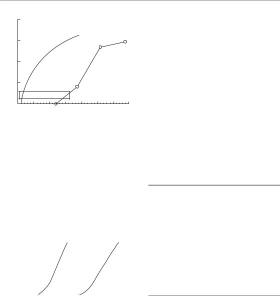
Figure 8.9 demonstrates the fit of the incomplete repair LQ model to data for pneumonitis in mice following fractionated thoracic irradiation with intervals of 3 hours between doses (Thames et al., 1984). The endpoint was mortality, expressed as the LD50 (radiation dose to produce lethality in 50 per cent of subjects). In these reciprocal-dose plots, incomplete repair makes the data bow upwards away from the straight line (dashed), which shows the pure LQ relationship that would be obtained when there is complete repair between successive doses, as would be the case with long time-intervals between fractions. An estimate of the repair halftime can be found by fitting data of the type shown in Figs 8.8 and 8.9 with the incomplete repair LQ model and seeking the T1/2 value that gives the best fit.

Dose per fraction (Gy)

Figure 8.9 Reciprocal dose plot (compare Fig. 8.5a) of data for pneumonitis in mice produced by fractionated irradiation; the points derive from experiments with different dose per fraction (and therefore different fraction numbers), always with 3 hours between doses. The upward bend in the data illustrates lack of sparing because of incomplete repair. From Thames et al. (1984), with permission.

Continuous irradiation

Another common situation in which incomplete repair occurs in clinical radiotherapy is during continuous irradiation. As described in Chapter 12, irradiation must be given at a very low dose rate (below about 5 cGy/hour) for full repair to occur during irradiation. At the other extreme, a single irradiation at high dose rate may not allow any significant repair to occur during exposure. As the dose rate is reduced below the high dose-rate range used in external-beam radiotherapy, the duration of irradiation becomes longer and the induction of DNA damage is counteracted by repair, leading to an increase in the isoeffective dose. The corresponding EQD2 formula for continuous irradiation incorporates a factor g to allow for incomplete repair:

where D is the total dose ( dose rate time). The parameter d is retained, as in the equation for fractionated radiotherapy, in order to deal with fractionated low dose-rate exposures. For a single

continuous exposure d D. This equation assumes that there is full recovery between the low dose-rate exposures; if not, the Hm factor must also be added (see Appendix). Table 8.3 gives values of the g factor for exposure times between 1 hour and 4 days.

The simple LQ model has also been applied to, for example, permanent interstitial implants and to biologically targeted radionuclide therapy. The interested reader is referred to the book by Dale and Jones (2007) listed under Further reading.

8.9 SHOULD A TIME FACTOR BE INCLUDED?

If the overall duration of fractionated radiotherapy is increased there will usually be greater repopulation of the irradiated tissues, both in the tumour and in early-reacting normal tissues. So far, we have not discussed the change in total dose necessary to compensate for changes in the overall duration of treatment. Overall time was included in the now-obsolete NSD and TDF models but is not put into the basic LQ approach described above. The reason for this is because the time factor in radiotherapy is now perceived to be more complex than had previously been supposed. For example, Fig. 8.10 shows that the extra dose needed to counteract proliferation in mouse skin does not become significant until about 2 weeks after the start of daily fractionation. In this and other situations, the time factor in the old NSD formula

(Fig. 8.10; broken line: total dose T 0.11) gives a false picture because it predicts a large amount of sparing if the overall time was increased from 1 to 12 days. These wrong time factors also underestimate the dose required to compensate for planned or unplanned gaps in treatment. Thus a T 0.11 factor predicts only an 8 per cent increase in total dose for a doubling of overall time, for example from 3.5 to 7 weeks. This would correspond to a 5.6 Gy increase in the total dose for a schedule delivering, say, 70 Gy to a squamous cell carcinoma of the head and neck. Clinical data summarized in Chapter 9 suggest that in this tumour type an additional dose of 16 Gy will be required to compensate for a 3.5-week prolongation of treatment time.

The use of the LQ model in clinical practice with no time factor at all is probably the best strategy for late-reacting tissues because any extra dose

Time after first fraction (days)

Figure 8.10 Extra dose required to counteract proliferation in mouse skin. Test doses of radiation were given at various intervals after a priming treatment with fractionated radiation. Proliferation begins about 12 days after the start of irradiation and is then equivalent to an extra dose of approximately 1.3 Gy/day. The broken line shows the prediction of the nominal standard dose (NSD) equation. Data from Denekamp (1973).