


5
Dose–response relationships in radiotherapy
SØREN M. BENTZEN
5.1 |
Introduction |
56 |
5.7 |
Methodological problems in estimating |
|
5.2 |
Shape of the dose–response curve |
57 |
|
dose–response relationships from clinical data |
64 |
5.3 |
Position of the dose–response curve |
59 |
5.8 |
Clinical implications: modifying the |
|
5.4 |
Quantifying the steepness of |
|
|
steepness of dose–response curves |
64 |
|
dose–response curves |
60 |
5.9 |
Normal tissue complication |
|
5.5 |
Clinical estimates of the steepness of |
|
|
probability (NTCP) models |
65 |
|
dose–response curves |
61 |
Key points |
66 |
|
5.6 |
The therapeutic window |
63 |
Bibliography |
66 |
|
|
|
|
|
|
|
5.1 INTRODUCTION
Clinical radiobiology is concerned with the relationship between a given physical absorbed dose and the resulting biological response and with the factors that influence this relationship. Although the term tolerance is frequently (mis-)used when discussing radiotherapy toxicity, it is important to realize that there is no dose below which the complication rate is zero: there is no clear-cut limit of tolerance. What is seen in clinical practice is a broad range of doses where the risk of a specific radiation reaction increases from 0 per cent towards 100 per cent with increasing dose (i.e. a dose–response relationship).
An endpoint is a specific event that may or may not have occurred at a given time after irradiation. The idea of dose–response is almost built into our definition of a radiation endpoint: to classify a biological phenomenon as a radiation effect we would require that this phenomenon be never or rarely seen after zero dose and seen in nearly all cases after very high doses. Various ways to characterize normal-tissue endpoints are discussed more fully
in Chapter 13 and tumour-related end-points are described in Chapter 7.
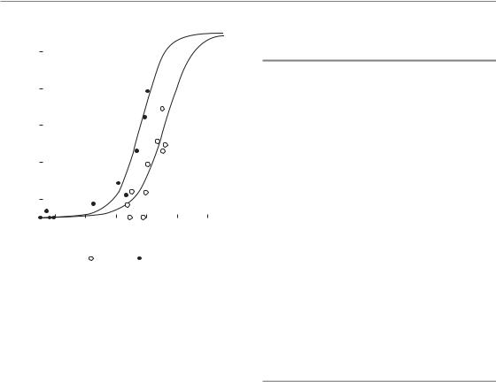
With increasing radiation dose, radiation effects may increase in severity (i.e. grade), in frequency (i.e. incidence) or both. A plot of, say, stimulated growth hormone secretion after graded doses of cranial irradiation in children may reveal an example of severity increasing with dose. Here we will concentrate on the other type of dose– response relationship: dose–incidence curves. In the same example we can obtain a dose–incidence curve by plotting the proportion of children with growth hormone secretion below a certain threshold as a function of dose. Thus, the dependent variable in a dose–response plot is an incidence or a probability of response as a function of dose (Fig. 5.1).
In this chapter we will introduce some key concepts in the quantitative description of dose– response relationships. Many of these ideas are important in understanding the general principles of radiotherapy. Furthermore, they form the basis of most of the more theoretical considerations in radiotherapy. We will keep the mathematics to a
Shape of the dose–response curve 57
(%) |
100 |
|
|
|
|
|
|
|
|
|
|
|
|
|
|
||
|
|
|
|
|
|
|
|
|
telangiectasia |
80 |
|
Assuming |
|||||
|
|
|||||||
|
|
|
RBE |
|||||
severeof |
60 |
|
|
|
|
|
|
|
|
|
|
|
|
|
|
||
40 |
|
|
|
|
|
|
|
|
Incidence |
|
|
|
|
|
|
|
|
20 |
|
|
|
|
|
|
|
|
|
|
|
|
|
|
|
|
|
|
0 |
|
|
|
|
|
|
|
|
|
|
|
|
|
|
|
|
|
|
|
|
|
|
|
|
|
15 |
25 |
35 |
45 |
55 |
|
65 |
75 |
|
|
|
Dose in 22-fractions (Gy) |
|
|
||||
|
|
|
|
|
|
|
|
|
|
|
|
Electron |
Photon |
|
|
|
|
|
|
|
|
|
|
|
|
|
Figure 5.1 Examples of dose–response relationships in clinical radiotherapy. Data are shown on the incidence of severe telangiectasia following electron or photon irradiation. RBE, relative biological effectiveness. From Bentzen and Overgaard (1991), with permission.
minimum but a few formulae are needed to substantiate the presentation.
Empirical attempts to establish dose–response relationships in the clinic date back to the first decade of radiotherapy. In 1936 the great clinical scientist Holthusen was the first to present a theoretical analysis of dose–response relationships and this has had a major impact on the conceptual development of radiotherapy optimization. Holthusen demonstrated the sigmoid shape of dose–response curves both for normal-tissue reactions (i.e. skin telangiectasia) and local control of skin cancer. He noted the resemblance between these curves and the cumulative distribution functions known from statistics, and this led him to the idea that the dose–response curve simply reflected the variability in clinical radioresponsiveness of individual patients. This remains one of the main hypotheses on the origin of dose–response relationships and this has had a renaissance in recent years with the growing interest in patient-to-patient variability in response to radiotherapy.
5.2 SHAPE OF THE DOSE–RESPONSE CURVE
Radiation dose–response curves have a sigmoid (i.e. ‘S’) shape, with the incidence of radiation effects tending to zero as dose tends to zero and tending to 100 per cent at very large doses. Many mathematical functions could be devised with these properties, but three standard formulations are used: the Poisson, the logistic and the probit dose–response models (Bentzen and Tucker, 1997). The first two are most frequently used and we will concentrate on these. In principle, it is an empirical problem to decide whether one model fits observed data better than the other. In reality, both clinical and experimental dose–response data are too noisy to allow statistical discrimination between these models and in most cases they will give very similar fits to a dataset. The situation where major discrepancies may arise is when these models are used for extrapolation of experience over a wide range of dose.
The Poisson dose–response model
Munro and Gilbert (1961) published a landmark paper in which they formulated the target-cell hypothesis of tumour control: ‘The object of treating a tumour by radiotherapy is to damage every single potentially malignant cell to such an extent that it cannot continue to proliferate’. From this idea and the random nature of cell killing by radiation they derived a mathematical formula for the probability of tumour cure after irradiation of ‘a number of tumours each composed of N identical cells’. More precisely, they showed that this probability depends only on the average number of clonogens surviving per tumour.
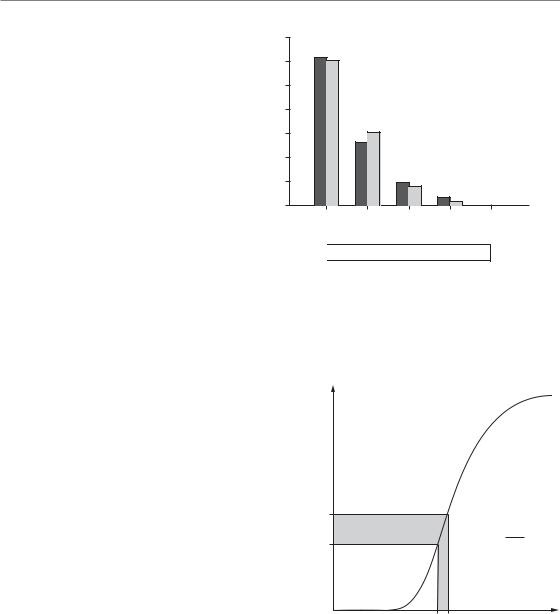
Figure 5.2 shows a Monte Carlo (i.e. random number) simulation of the number of surviving clonogens per tumour in a hypothetical sample of 100 tumours with an average number of 0.5 surviving clonogens per tumour. In Fig. 5.2a each tumour is represented by one of the squares in which the figure indicates the actual number of surviving clonogens, these numbers having been generated at random. The cured tumours are those with zero surviving clonogens. In this
58 Dose–response relationships in radiotherapy
0 |
0 |
0 |
2 |
1 |
1 |
1 |
0 |
0 |
0 |
0 |
0 |
0 |
0 |
0 |
0 |
0 |
0 |
1 |
0 |
0 |
0 |
0 |
2 |
1 |
2 |
1 |
2 |
0 |
1 |
1 |
0 |
0 |
0 |
0 |
2 |
1 |
0 |
1 |
2 |
1 |
2 |
0 |
0 |
0 |
0 |
0 |
0 |
0 |
3 |
0 |
0 |
0 |
0 |
0 |
0 |
0 |
1 |
1 |
0 |
1 |
0 |
2 |
0 |
0 |
0 |
0 |
0 |
0 |
1 |
0 |
0 |
0 |
0 |
0 |
3 |
0 |
0 |
1 |
0 |
0 |
3 |
1 |
1 |
1 |
1 |
0 |
0 |
0 |
1 |
0 |
1 |
2 |
1 |
1 |
0 |
0 |
1 |
1 |
0 |
|
|
|
|
|
|
|
|
|
|
(a)
|
70 |
|
|
|
|
(%) |
60 |
|
|
|
|
|
|
|
|
|
|
of ‘tumours’ |
50 |
|
|
|
|
40 |
|
|
|
|
|
30 |
|
|
|
|
|
Proportion |
|
|
|
|
|
20 |
|
|
|
|
|
10 |
|
|
|
|
|
|
0 |
|
|
|
|
|
0 |
1 |
2 |
3 |
4 |
|
|
Number of clonogens |
|
||


 ‘Observed’
 Predicted
(b)
Figure 5.2 Simulation of a Poisson distribution. (a) The number of clonogens surviving per tumour in a hypothetical sample of 100 tumours. The average number was 0.5 surviving clonogens per tumour. (b) Histogram shows the proportion of tumours with a given number of surviving clonogens (black bars) and this is compared with the prediction from a Poisson distribution with the same average number of surviving clonogens (grey bars).
simulation, there were 62 cured tumours. The relative frequencies of tumours with 0, 1, 2, . . .
surviving clonogens follow closely a statistical distribution known as the Poisson distribution, as shown in Fig. 5.2b. Many processes involving the counting of random events are (approximately) Poisson distributed, for example the number of decaying atoms per second in a radioactive sample or the number of tumour cells forming colonies in a Petri dish.
When describing tumour cure probability (TCP) it is the probability of zero surviving clonogens in a tumour that is of interest. This is the zero-order term of the Poisson distribution and if λ denotes the average number of clonogens per tumour after irradiation this is simply:
Response
γn |
|
D |
Dose
TCP e λ |
(5.1) |
Munro and Gilbert went one step further: they assumed that the average number of surviving clonogenic cells per tumour was a (negative) exponential function of dose. Under these assumptions they obtained the characteristic sigmoid dose–response curve (Fig. 5.3). Thus the shape of this curve could be explained solely from the random nature of cell killing (or clonogen
Figure 5.3 Geometrical interpretation of γ. A 1 per cent dose increment ( D) from a reference dose D yields an increase in response equal to γ percentage points. From Bentzen (1994), with permission.
survival) after irradiation: there was no need to assume variability of sensitivity between tumours.
The Poisson dose–response model derived by Munro and Gilbert has had a strong influence on

Position of the dose–response curve 59
theoretical radiobiology. The simple exponential dose–survival curve was later replaced by the linear-quadratic (LQ) model (see Chapters 4.10 and 8.4) and thus we arrive at what could be called the standard model of local tumour control:
TCP exp[ N0 exp( αD βdD)] (5.2)
Here, N0 is the number of clonogens per tumour before irradiation and the second exponential is simply the surviving fraction after a dose D given with dose per fraction d according to the LQ model. Thus when we multiply these two quantities we obtain the (average) number of surviving clonogens per tumour and this is inserted into the Poisson expression in equation 5.1. N0 can easily be expressed as a function of tumour volume and the clonogenic cell density (i.e. clonogens/cm3 of tumour tissue) and similarly it is easy to introduce exponential growth, with or without a lag time before accelerated repopulation, in this model. The immediate attraction of the Poisson model is that the model parameters appear to have a biological or mechanistic interpretation. This, however, is much less of a theoretical advantage than it appeared to be just 20 years ago. There are at least two reasons for this. First, it turns out that the model parameter estimates will be influenced by biological and dosimetric heterogeneity and therefore cannot usually be regarded as realistic measures of some intrinsic biological property of the tumour (Bentzen et al., 1991; Bentzen, 1992). Second, the model parameters have no simple interpretation in case of nor- mal-tissue effects where the radiation pathogenesis is more complex than suggested by the simple target cell model (Bentzen, 2006).
The logistic dose–response model
The logistic model is often introduced and used with more pragmatism than the Poisson model. This model has no simple mechanistic background and consequently the estimated parameters have no simple biological interpretation. Yet it is a convenient and flexible tool for estimating response probabilities after various exposures and is widely used in areas of biology other than
radiobiology. The idea of the model is to write the probability of an event (P) as:
P |
|
exp(u) |
(5.3) |
|
exp(u) |
||
1 |
|
||
where, when analysing data from fractionated radiotherapy, u has the form:
u a0 a1 D a2 D d |
(5.4) |
Here, D is total dose and d is dose per fraction, and the representation of the effect of dose fractionation in this way is of course reflecting the assumption of a LQ relationship between dose and effect. Additional terms, representing other patient or treatment characteristics, may be included in the model to see if they have a significant influence on the probability of effect. The coefficients a0, a1, . . .
are estimated by logistic regression, a method that is available in many standard statistical software packages. The parameters a1 and a2 play a role similar to the coefficients α and β of the linearquadratic model. But note that the mechanistic interpretation is not valid: a1 is not an estimate of αand a2 is not an estimate of β. What is preserved is the ratio a1/a2, which is an estimate of α/β.
Rearrangement of equation 5.3 yields the expression:
|
P |
|
|
|
|
|
|
|
|
u ln |
|
|
|
(5.5) |
|
|
|
|
|
1 |
P |
|
||
The ratio of P to (1 P) is called the odds of a response, and the natural logarithm of this is called the logit of P. Therefore, logistic regression is sometimes called logit analysis.
5.3 POSITION OF THE DOSE–RESPONSE CURVE
Several descriptors are used for the position of the dose–response curve on the radiation dose scale. They all have the unit of dose (Gy) and they specify the dose required for a given level of tumour control or normal-tissue complications. For tumours, the most frequently used position parameter is the TCD50 (i.e. the radiation dose for

60 Dose–response relationships in radiotherapy
50 per cent tumour control). For normal-tissue reactions, the analogous parameter is the radiation dose for 50 per cent response (RD50) or in the case of rare (severe) complications RD5, that is, the dose producing a 5 per cent incidence of complications.
5.4 QUANTIFYING THE STEEPNESS OF DOSE–RESPONSE CURVES
The most convenient way to quantify the steepness of the dose–response curve is by means of the ‘γ-value’ or, more precisely, the normalized dose–response gradient (Brahme, 1984; Bentzen and Tucker, 1997). This measure has a very simple interpretation, namely the increase in response in percentage points for a 1 per cent increase in dose. (Note: an increase in response from, say, 10 per cent to 15 per cent is an increase of 5 percentage points, but a 50 per cent relative increase). Figure 5.3 illustrates the definition of γ geometrically.
A more precise definition of γ requires a little mathematics. Let P(D) denote the response as a function of dose, D, and D a small increment in dose, then the ‘loose definition’ above may be written:
γ |
P(D D) P(D) |
100% |
|
|
||
|
|
|
||||
( |
D / D) 100% |
|
|
|||
D |
P(D D) P(D) |
D |
P |
(5.6) |
||
|
|
|||||
|
|
D |
D |
|||
The second term on the right-hand side is recognized as a difference-quotient, and in the limit where D tends to zero, we arrive at the formal definition of γ:
γ D P (D) |
(5.7) |
where P (D) is the derivative of P(D) with respect to dose.
If we look at the right-hand side of equation 5.6, we arrive at the approximate relationship:
P γ D |
(5.8) |
D |
|
In other words, γ is a multiplier that converts a relative change in dose into an (absolute) change
in response probability. Most often we insert the relative change in dose in per cent and in that case P is the (approximate) change in response rate in percentage points. This relationship is very useful in practical calculations (see Chapter 9, Section 9.10). For example, increasing the dose from 64 to 66 Gy in a schedule employing 2 Gy dose per fraction corresponds to a 3.1 per cent increase in dose. If we assume that the γ-value is 1.8, this yields an estimated improvement in local control of 1.8 3.1 5.6 percentage points.
Mathematically, equation 5.8 corresponds to approximating the S-shaped dose–response curve by a straight line (the tangent of the dose–response curve). As discussed briefly below, this will only be a good approximation over a relatively narrow range of doses; exactly how narrow depends on the response level and the steepness of the dose–response curve.
Clearly, the value of γ depends on the response level at which it is evaluated: at the bottom or top of the dose–response curve a 1 per cent increase in dose will produce a smaller increment in response than on the steep part of the curve. This local value of γis typically written with an index indicating the response level, for example γ50 refers to the γ-value at a 50 per cent response level. A compact and convenient way to report the steepness of a dose–response curve is by stating the γ-value at the level of response where the curve attains its maximum steepness: at the 37 per cent response level for the Poisson curve and at the 50 per cent response level for the logistic model. From this single value and a measure of the position of the dose–response curve, the whole mathematical form of the dose–response relationship is specified (Bentzen and Tucker, 1997). In particular, the steepness at any other dose or response level can be calculated. Table 5.1 shows how the γ-value varies with the response level for logistic dose–response curves of varying steepness. Using Table 5.1, it is possible to estimate the relevant γ-value at, say, a 20 per cent response level for a curve where the γ50 is specified. Table 5.1 also provides a useful impression of the range of response (or dose) where the simple linear approximation in equation 5.8 will be reasonably accurate. Clearly, if we extrapolate between two response levels where the γ-value has changed markedly, the approximation of assuming a fixed value for γwill not be very precise.
Clinical estimates of the steepness of dose–response curves 61
Table 5.1 γ values as a function of the response level for logistic dose-response curves of varying steepness
|
Response level (%) |
|
|
|
|
|
|
|
|
|
|
|
|
|
|
|
|
|
|
|
|
|
|
|
|
|
|
|
|
|
|
|
γ50 |
10 |
20 |
|
|
30 |
|
|
|
|
40 |
|
|
|
50 |
|
|
|
|
60 |
|
|
|
|
|
70 |
|
|
|
80 |
90 |
||
1 |
0.2 |
0.4 |
|
|
0.7 |
|
|
|
|
0.9 |
|
|
|
1.0 |
|
|
|
|
1.1 |
|
|
|
|
|
1.0 |
|
|
|
0.9 |
0.6 |
||
2 |
0.5 |
1.1 |
|
|
1.5 |
|
|
|
|
1.8 |
|
|
|
2.0 |
|
|
|
|
2.0 |
|
|
|
|
|
1.9 |
|
|
|
1.5 |
0.9 |
||
3 |
0.9 |
1.7 |
|
|
2.3 |
|
|
|
|
2.8 |
|
|
|
3.0 |
|
|
|
|
3.0 |
|
|
|
|
|
2.7 |
|
|
|
2.1 |
1.3 |
||
4 |
1.2 |
2.3 |
|
|
3.2 |
|
|
|
|
3.7 |
|
|
|
4.0 |
|
|
|
|
3.9 |
|
|
|
|
|
3.5 |
|
|
|
2.8 |
1.6 |
||
5 |
1.6 |
3.0 |
|
|
4.0 |
|
|
|
|
4.7 |
|
|
|
5.0 |
|
|
|
|
4.9 |
|
|
|
|
|
4.4 |
|
|
|
3.4 |
2.0 |
||
|
|
3 |
|
|
|
|
|
|
|
|
|
|
|
|
|
|
|
|
|
|
|
Larynx |
|
|
|
|
|
|
|
|||
|
|
|
|
|
|
|
|
|
|
|
|
|
|
|
|
|
|
|
|
|
|
|
|
|
|
|
|
|
||||
|
|
|
|
|
|
|
|
|
|
|
|
|
|
|
|
|
|
|
|
|
|
Head and neck |
|
|
||||||||
|
|
|
|
|
|
|
|
|
|
|
|
|
|
|
|
|
|
|
|
|
|
Supraglottic |
|
|
|
|||||||
|
|
|
|
|
|
|
|
|
|
|
|
|
|
|
|
|
|
|
|
|
|
Pharynx |
|
|
|
|
|
|||||
|
|
2 |
|
|
|
|
|
|
|
|
|
|
|
|
|
|
|
|
|
|
|
Neck nodes |
|
|
|
|||||||
|
|
|
|
|
|
|
|
|
|
|
|
|
|
|
|
|
|
|
|
|
|
|
|
|
|
|
|
|
|
|
|
|
|
|
37 |
|
|
|
|
|
|
|
|
|
|
|
|
|
|
|
|
|
|
|
|
|
|
|
|
|
|
|
|
|
|
|
|
γ |
|
|
|
|
|
|
|
|
|
|
|
|
|
|
|
|
|
|
|
|
|
|
|
|
|
|
|
|
|
|
|
|
1 |
|
|
|
|
|
|
|
|
|
|
|
|
|
|
|
|
|
|
|
|
|
|
|
|
|
|
|
|
|
|
|
|
0 |
|
|
|
|
|
|
|
|
|
|
|
|
|
|
|
|
|
|
|
|
|
|
|
|
|
|
|
|
|
|
|
|
n |
C |
|
Sle |
|
|
|
|
ar |
ham |
|
T |
|
|
en |
|
oenc |
ham |
T |
|
|
ham |
|
|
|
|
ein |
|
hames |
|
|
|
|
|
|
|
|
|
|
|
|
|
|
|
|
|
|
|
|
|
|
|||||||||||||
|
|
e |
|
|
v |
|
|
|
|
|
es |
ars |
|
|
|
|
h |
es |
lor |
|
es |
|
es |
|
|
|
|
|
|
|||
|
|
|
|
|
|
|
|
|
r |
t |
|
|
|
|
r |
|
|
|
|
|
|
|
|
|
|
|
|
|
|
|
|
|
|
|
|
|
ohen |
|
|
ergaard |
|
t |
|
|
|
|
t |
|
|
|
|
|
|
|
|
|
|
|
|
|
|
|
|
|
|
|
|
n |
|
|
|
St |
ewa |
St |
|
|
ok |
St |
ewa |
|
|
|
|
|
ay |
Tham |
|
|
|
|
|
|
|
|
|
|
||
|
|
Ha |
|
|
|
|
|
|
|
|
|
|
|
|
|
|
|
|
|
|
|
|
|
|
||||||||
|
|
s |
|
|
|
|
|
|
|
|
T |
|
|
|
|
Bent |
M |
|
T |
|
|
|
T |
|
|
|
|
|
T |
|
|
|
|
|
|
|
|
|
|
|
|
|
|
|
|
|
|
z |
|
|
|
|
|
|
|
|
|
Ghos |
s |
Ghos |
s |
|
|
|
|
|
|
|
|
|
|
|
|
|
|
|
|
|
|
|
|
|
|
|
|
|
|
|
|
|
|
|
|
|
||||
|
|
– |
|
|
|
Ov |
|
|
|
|
|
|
|
|
|
|
|
|
|
|
|
|
|
|
|
|
|
|
|
|
||
|
|
lm |
|
|
|
|
|
|
|
|
|
|
|
|
|
|
|
|
|
|
|
|
|
|
|
|
|
|
|
|
|
|
|
|
Hje |
|
|
|
|
|
|
|
|
|
|
|
|
|
|
|
|
|
|
|
|
|
|
|
|
|
|
|
|
|
|
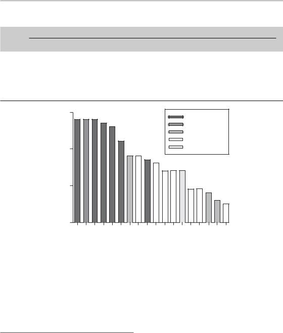
Figure 5.4 Estimated γ37 values from a number of studies on dose-response relationships for squamous cell carcinoma in various sites of the head and neck. From Bentzen (1994), where the original references may be found. Reprinted with permission from Elsevier.
5.5 CLINICAL ESTIMATES OF THE STEEPNESS OF DOSE–RESPONSE CURVES
Several clinical studies have found evidence for a significant dose–response relationship and have provided data allowing an estimation of the steepness of clinical dose–response curves. Clinical dose–response curves generally originate from studies where the dose has been changed while keeping either the dose per fraction or the number of fractions fixed. A further advantage of tabulating the γ-value at the steepest point of the dose–response curve is that it is independent of the
dose-fractionation details in the case of a dose–response curve generated using a fixed dose per fraction (Brahme, 1984). Figure 5.4 shows estimates of γ37 for head and neck tumours under the assumption of a fixed dose per fraction (Bentzen, 1994). Typical values range from 1.5–2.5. This means that, around the midpoint of the dose– response curve, for each per cent increment in dose, the probability of controlling a head and neck tumour will increase by 2 percentage points. Steepness estimates from dose–response curves for other tumour histologies have been reviewed by Okunieff et al. (1995), but it should be noted that data for other histologies are generally
62 Dose–response relationships in radiotherapy
|
7 |
|
|
|
|
|
|
|
|
|
|
|
|
|
|
|
|
|
|
|
|
|
|
|
|
|
|
|
|
|
|
|
|
Fixed number of fractions (22) |
||||||||||||||
|
|
|
|
|
|
|
|
|
|
|
|
|
|
|
|
|
|
|
|
|
|
|
|
|
|
|
|
|
|
|
|
|
|
|
||||||||||||||
|
6 |
|
|
|
|
|
|
|
|
|
|
|
|
|
|
|
|
|
|
|
|
|
|
|
|
|
|
|
|
|
|
|
|
Fixed dose per fraction |
||||||||||||||
|
|
|
|
|
|
|
|
|
|
|
|
|
|
|
|
|
|
|
|
|
|
|
|
|
|
|
|
|
|
|
|
|
|
|
|
|
|
|
|
|
|
|
|
|
|
|
||
|
5 |
|
|
|
|
|
|
|
|
|
|
|
|
|
|
|
|
|
|
|
|
|
|
|
|
|
|
|
|
|
|
|
|
|
|
|
|
|
|
|
|
|
|
|
|
|
|
|
50 |
4 |
|
|
|
|
|
|
|
|
|
|
|
|
|
|
|
|
|
|
|
|
|
|
|
|
|
|
|
|
|
|
|
|
|
|
|
|
|
|
|
|
|
|
|
|
|
|
|
|
|
|
|
|
|
|
|
|
|
|
|
|
|
|
|
|
|
|
|
|
|
|
|
|
|
|
|
|
|
|
|
|
|
|
|
|
|
|
|
|
|
|
|
|
|
|
|
|
γ |
3 |
|
|
|
|
|
|
|
|
|
|
|
|
|
|
|
|
|
|
|
|
|
|
|
|
|
|
|
|
|
|
|
|
|
|
|
|
|
|
|
|
|
|
|
|
|
|
|
|
|
|
|
|
|
|
|
|
|
|
|
|
|
|
|
|
|
|
|
|
|
|
|
|
|
|
|
|
|
|
|
|
|
|
|
|
|
|
|
|
|
|
|
|
|
|
||
|
2 |
|
|
|
|
|
|
|
|
|
|
|
|
|
|
|
|
|
|
|
|
|
|
|
|
|
|
|
|
|
|
|
|
|
|
|
|
|
|
|
|
|
|
|
|
|
Head and neck |
|
|
|
|
|
|
|
|
|
|
|
|
|
|
|
|
|
|
|
|
|
|
|
|
|
|
|
|
|
|
|
|
|
|
|
|
|
|
|
|
|
|
|
|
|
|
|
tumours |
||
|
|
|
|
|
|
|
|
|
|
|
|
|
|
|
|
|
|
|
|
|
|
|
|
|
|
|
|
|
|
|
|
|
|
|
|
|
|
|
|
|
|
|
|
|
|
|
|
|
|
1 |
|
|
|
|
|
|
|
|
|
|
|
|
|
|
|
|
|
|
|
|
|
|
|
|
|
|
|
|
|
|
|
|
|
|
|
|
|
|
|
|
|
|
|
|
|
|
|
|
0 |
|
|
|
|
|
|
ma |
|
|
|
|
|
|
|
r |
|
|
|
|
|
|
s |
|
|
|
|
|
a |
|
|
|
|
a |
|
|
|
|
|
|
e |
|
|
|
|
|
d |
|
|
|
|
|
|
|
|
|
|
|
|
|
|
|
|
e |
|
|
|
|
|
|
|
|
|
|
|
|
|
|
|
|
|
|
|
|
t |
|
|
|
|
i |
|||||||
|
|
|
|
|
|
|
|
e |
|
|
|
|
u |
l d |
|
|
|
|
|
|
ro |
si |
|
|
|
|
|
si |
|
|
|
|
si |
|
|
|
, |
l a |
|
|
|
|
mo |
|
||||
|
|
|
|
|
|
|
|
|
|
|
|
|
|
|
|
|
|
|
|
|
|
|
ct |
|
|
|
|
|
|
|
|
|
|
|
|
|
|
|||||||||||
|
|
|
|
|
o |
e |
d |
|
|
|
|
o |
|
|
|
|
|
|
|
fib |
|
|
|
|
i e |
|
|
|
|
i e |
ct |
|
|
n g |
|
|
|
|
|
g |
|
|
||||||
|
|
|
|
|
|
|
|
|
|
|
|
|
|
|
|
|
t. |
|
|
|
|
g |
|
|
|
g |
|
u |
|
|
|
|
|
|
|
|
|
|||||||||||
|
|
|
|
l |
|
|
|
|
|
|
|
|
|
|
|
|
|
|
|
|
|
|
|
|
|
|
|
|
|
|
|
|
|
|
|
|
||||||||||||
|
|
|
e a |
|
|
|
|
|
|
|
e n |
|
|
|
|
|
|
cu |
|
|
|
l a |
n |
|
|
|
l a |
n |
|
|
L |
|
|
|
|
|
|
ct |
o |
|
|
|
||||||
|
|
|
|
|
|
|
|
|
|
|
z |
|
|
|
|
|
u b |
|
|
|
Te |
|
|
|
Te |
|
|
|
|
|
|
|
|
|
R e |
|
|
|
||||||||||
|
|
|
|
|
|
|
|
|
|
ro |
|
|
|
|
|
|
|
|
|
|
|
|
|
|
|
|
|
|
|
|
|
|
|
|
|
|
|
|||||||||||
|
a |
r |
yn |
|
|
|
|
|
|
F |
|
|
|
|
|
S |
|
|
|
|
|
|
|
|
|
|
|
|
|
|
|
|
|
|
|
|
|
|
|
|
|
|
||||||
L |
|
|
|
|
|
|
|
|
|
|
|
|
|
|
|
|
|
|
|
|
|
|
|
|
|
|
|
|
|
|
|
|
|
|
|
|
|
|
|
|
|
|
||||||
|
|
|
|
|
|
|
|
|
|
|
|
|
|
|
|
|
|
|
|
|
|
|
|
|
|
|
|
|
|
|
|
|
|
|
|
|
|
|
|
|
|
|
|
|
|
|
||
|
|
|
|
|
|
|
|
|
|
|
|
|
|
|
|
|
|
|
|
|
|
|
|
|
|
|
|
|
|
|
|
|
|
|
|
|
|
|
|
|
|
|
|
|
|
|
|
|
Figure 5.5 Estimated γ50 values for various late normal-tissue endpoints. Estimates are shown for treatment with a fixed dose per fraction and a fixed number of fractions. The shaded horizontal band corresponds to the typical γ-values at the point of maximum steepness for dose-response curves in head and neck tumours. Compare with Fig. 5.4. Data from Bentzen (1994) and Bentzen and Overgaard (1996), where the original references may be found.
more sparse than for the head and neck tumours. Also, some estimated values are obviously outliers that cannot be taken as serious estimates of the steepness of the clinical dose–response curve. These extreme values must be explained by patient selection bias or errors in dosimetry.
In the absence of other sources of variation, the maximum steepness of a tumour-control curve is determined only by the Poisson statistics of survival of clonogenic cells (Fig. 5.2), and this should roughly give rise to a value of γ37 7 (Suit et al., 1992). However, values as high as this are not achieved even in transplantable mouse tumour models under highly controlled experimental conditions (Khalil et al., 1997). The principal reason why dose–response curves in the laboratory and in the clinic are shallower than this theoretical limit is dosimetric and biological heterogeneity. The tendency for vocal cord tumours to have γ37 values at the upper end of the interval seen for other head and neck subsites probably reflects the relatively lower heterogeneity among laryngeal carcinomas treated with radiotherapy. Other patient and treatment characteristics will influence both the position and the steepness of the dose–response curve. It can be shown (Brahme,
1984) that the γ37 of a Poisson dose–response curve for a fixed dose per fraction depends only on the number of clonogens that have to be sterilized to cure the tumour. As mentioned in Section 5.2, many tumour and treatment variables, for example tumour volume and overall treatment time, are thought to affect the (effective) number of clonogens to be sterilized. Therefore, in a multivariate analysis, γ37 will depend on all the significant patient and treatment characteristics.
Figure 5.5 shows a selection of γ50 values for normal-tissue endpoints. Estimates are given both for treatment with a fixed dose per fraction and, where possible, also for treatment in a fixed number of fractions, in this case 22. The estimates in the latter situation are considerably higher, which is as expected from the LQ model. The explanation is that, when treating with a fixed number of fractions, increasing the dose leads to a simultaneous increase in dose per fraction, and this is associated with an increased biological effect per gray. This is another manifestation of the ‘double trouble’ phenomenon discussed in Chapter 9, Section 9.11. Let γN denote the steepness of the dose–response curve for a fixed fraction number, and γd the

The therapeutic window 63
steepness for a fixed dose per fraction, then it can be shown that at a dose per fraction of dr:
γN γd |
(α/β) 2 dr |
(5.9) |
|
(α/β) dr |
|||
|
|
As both α/β and dr are positive numbers, γN is always larger than γd. In the limit of very large dose per fraction, γN has a limiting value of 2 γd. In the limit of dose per fraction tending to zero, γN tends to γd. For more discussion of equation 5.9 and its significance for dosimetric precision requirements in radiotherapy, see Bentzen (2005).
Figure 5.5 shows a spectrum of γ50 values for the various endpoints. The dose–response curves for many late endpoints are steeper than for head and neck cancer. An exception is rectosigmoid complications after combined external-beam and intracavitary brachytherapy where a large dose–volume heterogeneity is present because of the steep gradients in the dose distribution from the intracavitary sources. Also, the lung data arise from a treatment technique where the dose to the lung tissue was heterogeneous. Thus it is likely that dosimetric rather than intrinsic biological factors are the main cause of the relatively low steepness seen for these endpoints.
5.6 THE THERAPEUTIC WINDOW
As with any other medical procedure, prescription of a course of radiotherapy must represent a balance between risks and benefits. The relative position and shape of the dose–response curves for tumour control and a given radiotherapy complication determine the possibility of delivering a sufficient dose with an acceptable level of side-effects. This was nicely illustrated by Holthusen, who plotted dose–response curves for tumour control and complications in the same coordinate system for two hypothetical situations: one favourable, that is with a wide therapeutic window between the two curves, and the other one less favourable. Figure 5.6 shows an example of how changing treatment parameters may affect the therapeutic window. For split-course treatment (Fig. 5.6a) the tumour and oedema curves are closer together than for conventional treatment (Fig. 5.6b) and the therapeutic window is therefore narrower. In practice, there will
|
100 |
|
|
Split-course treatment |
|
|
|
|
|
|
|||||
|
|
|
|
|
|
|
|
||||||||
|
80 |
|
|
(10 weeks overall time) |
|
|
|
|
|
|
|||||
(%) |
|
|
|
|
|
|
Tumour |
|
|
|
|
|
|
||
|
|
|
|
|
|
|
|
|
|
|
|||||
60 |
|
|
|
|
|
|
|
|
|
|
|
|
|||
Response |
|
|
|
|
|
|
|
|
|
|
|
|
|||
|
|
|
|
|
|
|
|
|
|
|
|
|
|
||
40 |
|
|
|
|
|
|
|
|
|
Late oedema |
|||||
|
|
|
|
|
|
|
|
|
|
||||||
|
|
|
|
|
|
|
|
|
|
|
|||||
|
20 |
|
|
|
|
|
|
|
|
|
|
|
|
|
|
|
|
|
|
|
|
|
|
|
|
|
|
|
|
||
|
0 |
|
|
|
|
|
|
|
|
|
|
|
|
|
|
|
|
|
|
|
|
|
|
|
|
|
|
|
|
||
|
|
|
|
|
|
60 |
70 |
80 |
90 |
||||||
|
30 |
40 |
50 |
||||||||||||
(a) |
|
|
|
|
|
Radiation dose (Gy) |
|
|
|
|
|||||
|
100 |
|
|
Conventional treatment |
|
|
|
|
|
|
|||||
|
|
|
|
|
|
|
|
|
|||||||
|
80 |
|
|
(6 weeks overall time) |
|
|
|
|
|
|
|||||
(%) |
|
|
|
|
|
|
|
|
|
|
|
|
|
|
|
|
|
|
|
|
|
|
|
|
|
|
|
|
|
||
60 |
|
|
|
|
|
|
|
|
|
|
|
|
|
|
|
Response |
|
|
|
|
Tumour |
|
|
|
|
|
|
|
|
||
|
|
|
|
|
|
|
|
|
|
|
|
||||
|
|
|
|
|
|
|
|
|
|
|
|
|
|||
|
|
|
|
|
|
|
|
|
|
|
|
|
|
||
|
40 |
|
|
|
|
|
|
|
|
|
Late oedema |
|
|
||
|
|
|
|
|
|
|
|
|
|
|
|
||||
|
|
|
|
|
|
|
|
|
|
|
|
|
|||
|
20 |
|
|
|
|
|
|
|
|
|
|
|
|
|
|
|
|
|
|
|
|
|
|
|
|
|
|
|
|
|
|
|
0 |
|
|
|
|
|
|
|
|
|
|
|
|
|
|
|
|
|
|
|
|
|
|
|
|
|
|
|
|
|
|
|
30 |
40 |
50 |
60 |
70 |
80 |
90 |
||||||||
(b) |
|
|
|
|
|
Radiation dose (Gy) |
|
|
|
|
|||||
Figure 5.6 Dose–response curves for local control of laryngeal carcinoma (solid lines) and late laryngeal oedema as estimated from the data by Overgaard et al. (1988). Protraction of overall treatment time narrowed the therapeutic window. From Bentzen and Overgaard (1996), with permission.
be several sequelae of clinical concern and each of these will have its characteristic dose–response curve and will respond differently to treatment modifications. This complicates the simple strategy for optimization suggested by Fig. 5.6.
Several parameters are found in the literature for quantifying the effect of treatment modifications on the therapeutic window. Holthusen’s proposal was to calculate the probability of uncomplicated cure, and this is still used frequently in the literature. The difficulty with this measure is that it gives equal weight to the complication in question and to tumour recurrence, which may often be fatal, and this is against common sense. A simple alternative, which is easy to interpret but not necessarily easy to estimate from an actual dataset, is to specify the tumour control probability at isotoxicity with respect to a specific end-point, as illustrated in Fig. 1.3.

64 Dose–response relationships in radiotherapy
5.7 METHODOLOGICAL PROBLEMS IN ESTIMATING DOSE–RESPONSE RELATIONSHIPS FROM CLINICAL DATA
An increasing number of publications are concerned with the quantitative analysis of clinical radiobiological data. Many methodological problems must be addressed in such studies and these problems may roughly be grouped as clinical, dosimetric and statistical.
●Clinical aspects – these include the evaluation of well-defined endpoints for tumour and nor- mal-tissue effects. Endpoints requiring prolonged observation of the patients, such as local tumour control or late complications, should be analysed using actuarial statistical methods. Special concerns exist for evaluation, grading and reporting of injury to normal tissue and these are discussed in Chapter 13, Section 13.4. For dose–response data obtained from non-randomized studies, the reasons for variability in dose should be carefully considered. Subsets of patients treated with low/high doses may not be comparable in terms of other patient characteristics influencing the outcome. An example is where patients receive a lower total dose than prescribed because of their poor general condition, perhaps in combination with severe early reactions, or because of progressive disease during treatment.
●Dosimetric aspects – these involve a detailed account of treatment technique and quality assurance procedures employed. Furthermore, the identification of biologically relevant dosimetric reference points and a proper evaluation of the doses to these points are required. Modern radiation therapy techniques often give rise to a highly non-uniform dose distribution in the relevant normal tissues. This distribution will have to be converted into an equivalent dose, or similar quantity.
●Statistical aspects – these include the choice of valid statistical methods that are appropriate for the data type in question and which use the available information in an optimal way. Statistical tests for significance or, preferably, confidence limits on estimated parameters should be specified. When negative findings are reported, an assessment of the statistical power
of the study should be given. Finally, the censoring (i.e. incomplete follow-up) and latency should be allowed for.
For an overview of the quantitative analysis of clinical data, see Bentzen (1993) and Bentzen et al. (2003).
5.8 CLINICAL IMPLICATIONS: MODIFYING THE STEEPNESS OF DOSE–RESPONSE CURVES
The γ-value is not only useful as a multiplier in converting from a dose change to a change in response but may also be used as a multiplier for converting an uncertainty in dose into an uncertainty in response. If the standard deviation of the absorbed-dose distribution in a population of patients is 5 per cent, a γ-value of 3 would yield an estimated 15 per cent standard deviation on the response-probability distribution. Note that in this situation it is generally the γ for a fixed number of fractions that applies. Figure 5.5 shows that the high γ-values at the maximum steepness of the dose–response curve for normal tissues would yield a large variability in response probability for a 5 per cent variability in absorbed dose. This provides an indication of the precision required in treatment planning and delivery in radiotherapy.
Another field where the steepness of the dose–response curves for tumours and normaltissue reactions plays a crucial role is in the design of clinical trials. For a discussion of this topic see Bentzen (1994).
A final issue in this chapter is the prospect for modifying the steepness of the clinical dose–response curve. Several modelling studies have shown that patient-to-patient variability in tumour biological parameters could strongly affect the steepness of the dose–response curve (Bentzen et al., 1990; Bentzen, 1992; Suit et al., 1992; Webb and Nahum, 1993). Compelling support for this idea also comes from experimental studies (Khalil et al., 1997). A direct illustration of the effect of interpatient variability is obtained from an analysis of local tumour control in patients with oropharyngeal cancers (Bentzen,
1992). Analysing the data with the Poisson model yielded γ37 1.8. An analysis taking an assumed
Normal tissue complication probablility (NTCP) models 65
|
100 |
10% 20% |
50% |
80% |
|
|
|
90% |
|
|
|
|
|
|
|
80 |
|
|
|
(%) |
60 |
|
|
|
control |
|
|
|
|
|
|
|
|
|
Local |
40 |
|
|
|
|
|
|
|
|
|
20 |
|
|
|
|
0 |
60 |
80 |
100 |
|
40 |
Biological dose (Gy)
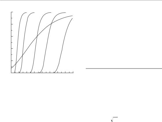
Figure 5.7 Local control of oropharyngeal carcinoma as a function of the biological dose in 2-Gy fractions. Dotted lines are theoretical dose–response curves after stratification for intrinsic radiosensitivity. These represent dose–response relationships from five homogeneous patient populations with radiosensitivity equal to selected percentiles of the radiosensitivity distribution in the total population. From Bentzen (1994), with permission.
variability in tumour cell radiosensitivity into account allowed the dose–response curve to be broken down into a series of very steep curves, each of which would apply to a subpopulation of patients stratified according to intrinsic radiosensitivity (Fig. 5.7). Clinical data on pathological response after radiotherapy analysed by Levegrün et al. (2002) showed how the dose–incidence curve got steeper when stratifying patients according to clinico-pathological risk group. Also, for normaltissue effects, adjustment for patient-related risk factors leads to a steeper dose–response curve (Honore et al., 2002).
This interpatient variability also has a major influence on the parameter estimates in the Poisson model (Bentzen, 1992). Fenwick (1998) proposed a closed form expression of the Poisson dose–response model that takes patient-to-patient variability explicitly into account, but this approach has only been used in a few analyses so far. For a detailed discussion of interpatient variability
and dose–response analysis, see Roberts and Hendry (2007).
Viewing these curves in relation to Fig. 5.6, it is clear that some of these subgroups could be expected to have a greater therapeutic window than others. If, by means of a reliable predictive assay, these subgroups could be identified before starting therapy, a substantial therapeutic benefit could be realized.
5.9 NORMAL TISSUE COMPLICATION PROBABILITY (NTCP) MODELS
Several dose–volume models for normal tissues have been proposed in the literature [see the recent reviews by Yorke (2001) and Kong et al. (2007)]. The most widely used of these is the Lyman model (Lyman, 1985). This model gives the normal tissue complication probability (NTCP), as a function of the absorbed dose, D, in a partial organ volume, V:
NTCP(D,V ) |
1 |
∫ u(D,V ) exp( 1 |
x2 )dx |
|
2π |
||||
|
2 |
|
||
|
|
|
(5.10) |
where the dependence of dose and volume is in the upper limit of the integral:
u(D,V ) |
D D50 (V ) |
(5.11) |
m D (V ) |
|
|
50 |
|
|
The volume dependence of the D50 is assumed to follow the relationship:
D (V ) |
D50 (1) |
(5.12) |
50 |
V n |
|
A closer inspection of these three equations shows that there are two independent variables, D and V, and three model parameters, m, D50(1) and n. D50(1) is the uniform total dose producing a 50 per cent incidence of the specific endpoint if the whole organ is receiving this dose. The volume exponent, n, is always between zero and 1 and the larger the value, the more pronounced is the volume effect. The third parameter, m, is inversely related to the steepness of the dose–response curve (i.e. smaller values of m correspond to steeper

66 Dose–response relationships in radiotherapy
dose–response curves). The Lyman model has no simple mechanistic background but should be seen as a flexible empirical model for fitting dose–vol- ume datasets. Attempts have been made to develop more mechanistic models but it is questionable whether the biological complexity of dose–volume effects can be encompassed in a reasonably simple mathematical model and most often these models are applied in a pragmatic way as a simple means of capturing the main effects of dose and volume.
Lyman’s model only applies to fractional volumes receiving uniform doses. In practice, this is rarely (read: never!) the case. The most common way of summarizing information on a non-uni- form dose distribution in an organ is the dose–vol- ume histogram (DVH). In order to estimate the NTCP from a DVH using the Lyman model, it is necessary to reduce the DVH into a single point in dose–volume space. The most frequently used method for doing this is the effective volume method (Kutcher and Burman, 1989) whereby the DVH is transformed into an equivalent fractional volume receiving the maximum dose in the DVH. The basic assumption of this method is that each fractional volume will follow the same dose– volume relationship (described by the Lyman model) as the whole organ. The partial volume in a specific bin on the dose axis is then converted into a (smaller) volume placed at the bin corresponding to the maximum absorbed dose in the DVH.
Some caveats should be noted regarding the use of NTCP models in clinical radiotherapy. Studies have shown that models fitted to one clinical dataset may have low predictive power when applied to an independent data series (Bradley et al., 2007). Also, patients receiving cytotoxic chemotherapy may require tighter dose–volume constraints in order to have a risk similar to that of patients treated with radiation alone (Bradley et al., 2004). Finally, it should be noted that most models used so far have been based on analysis of the DVH alone; in other words, they do not consider the actual spatial distribution of dose in the organ at risk. One example where this analytic strategy seems to break down is the lung, where there are quite good data suggesting that the functional importance of damage to a subvolume of a given size depends on its location within the lung (Travis et al., 1997; Bradley et al., 2007).
Therefore, NTCP models should at present not be used in clinical decision-making and in doseplanning outside a research setting.
Key points
1.There is no well-defined ‘tolerance dose’ for radiation complications or ‘tumouricidal dose’ for local tumour control: rather, the probability of a biological effect rises from 0 per cent to 100 per cent over a range of doses.
2.The steepness of a dose–response curve at a
response level of n per cent may be quantified by the value γn, that is the increase in response in percentage points for a 1 per cent increase in dose.
3.Dose–response curves for late normal-tis- sue endpoints tend to be steeper (typical γ50 between 2 and 6) than the dose–response
curves for local control of squamous cell carcinoma of the head and neck (typical γ50 between 1.5 and 2.5).
4.The steepness of a dose–response curve is higher if the data are generated by varying the dose while keeping the number of fractions constant (‘double trouble’) than if the dose per fraction is fixed.
5.Dosimetric and biological heterogeneity cause the population dose–response curve to be more shallow.
6.Normal-tissue complication probability models, incorporating dose fractionation as well as irradiated volume, have not been validated in any clinical setting and should not be routinely used outside a research protocol.
■BIBLIOGRAPHY
Bentzen SM (1992). Steepness of the clinical dosecontrol curve and variation in the in vitro radiosensitivity of head and neck squamous cell carcinoma. Int J Radiat Biol 61: 417–23.
Bentzen SM (1993). Quantitative clinical radiobiology.
Acta Oncol 32: 259–75.
Bentzen SM (1994). Radiobiological considerations in the design of clinical trials. Radiother Oncol 32: 1–11.

Bibliography 67
Bentzen SM (2005). Steepness of the radiation dose–response curve for dose-per-fraction escalation keeping the number of fractions fixed.
Acta Oncol 44: 825–8.
Bentzen SM (2006). Preventing or reducing late side effects of radiation therapy: radiobiology meets molecular pathology. Nat Rev Cancer 6: 702–13.
Bentzen SM, Overgaard M (1991). Relationship between early and late normal-tissue injury after postmastectomy radiotherapy. Radiother Oncol 20: 159–65.
Bentzen SM, Overgaard J (1996). Clinical normal tissue radiobiology. In: Tobias JS, Thomas PRM(eds) Current radiation oncology. London: Arnold, 37–67.
Bentzen SM, Tucker SL (1997). Quantifying the position and steepness of radiation dose–response curves. Int J Radiat Biol 71: 531–42.
Bentzen SM, Thames HD, Overgaard J (1990). Does variation in the in vitro cellular radiosensitivity explain the shallow clinical dose-control curve for malignant melanoma? Int J Radiat Biol 57: 117–26.
Bentzen SM, Johansen LV, Overgaard J, Thames HD (1991). Clinical radiobiology of squamous cell carcinoma of the oropharynx. Int J Radiat Oncol Biol Phys 20: 1197–206.
Bentzen SM, Dorr W, Anscher MS et al. (2003). Normal tissue effects: reporting and analysis. Semin Radiat Oncol 13: 189–202.
Bradley J, Deasy JO, Bentzen S, El-Naqa I (2004). Dosimetric correlates for acute esophagitis in patients treated with radiotherapy for lung carcinoma. Int J Radiat Oncol Biol Phys 58: 1106–13.
Bradley JD, Hope A, El Naqa I et al. (2007). A nomogram to predict radiation pneumonitis, derived from a combined analysis of RTOG 9311 and institutional data. Int J Radiat Oncol Biol Phys 69: 985–92.
Brahme A (1984). Dosimetric precision requirements in radiation therapy. Acta Radiol Oncol 23: 379–91.
Fenwick JD (1998). Predicting the radiation control probability of heterogeneous tumour ensembles: data analysis and parameter estimation using a closed-form expression. Phys Med Biol 43: 2159–78.
Honore HB, Bentzen SM, Moller K, Grau C (2002). Sensori-neural hearing loss after radiotherapy for nasopharyngeal carcinoma: individualized risk estimation. Radiother Oncol 65: 9–16.
Khalil AA, Bentzen SM, Overgaard J (1997). Steepness of the dose–response curve as a function of volume in an experimental tumor irradiated under ambient or
hypoxic conditions. Int J Radiat Oncol Biol Phys 39: 797–802.
Kong FM, Pan C, Eisbruch A, Ten Haken RK (2007). Physical models and simpler dosimetric descriptors of radiation late toxicity. Semin Radiat Oncol 17: 108–20.
Kutcher GJ, Burman C (1989). Calculation of complication probability factors for non-uniform normal tissue irradiation: the effective volume method. Int J Radiat Oncol Biol Phys 16: 1623–30.
Levegrün S, Jackson A, Zelefsky MJ et al. (2002). Risk group dependence of dose–response for biopsy outcome after three-dimensional conformal radiation therapy of prostate cancer. Radiother Oncol 63: 11–26.
Lyman JT (1985). Complication probability as assessed from dose–volume histograms. Radiat Res Suppl 8: S13–9.
Munro TR, Gilbert CW (1961). The relation between tumour lethal doses and the radiosensitivity of tumour cells. Br J Radiol 34: 246–51.
Okunieff P, Morgan D, Niemierko A, Suit HD (1995). Radiation dose–response of human tumors. Int J Radiat Oncol Biol Phys 32: 1227–37.
Overgaard J, Hjelm-Hansen M, Johansen LV, Andersen AP (1988). Comparison of conventional and split-course radiotherapy as primary treatment in carcinoma of the larynx. Acta Oncol 27: 147–52.
Roberts SA, Hendry JH (2007). Inter-tumour heterogeneity and tumour control. In: Dale R, Jones B (eds) Radiobiological modelling in radiation oncology. London: British Institute of Radiology, 169–95.
Suit H, Skates S, Taghian A, Okunieff P, Efird JT (1992). Clinical implications of heterogeneity of tumor response to radiation therapy. Radiother Oncol 25: 251–60.
Travis EL, Liao ZX, Tucker SL (1997). Spatial heterogeneity of the volume effect for radiation pneumonitis in mouse lung. Int J Radiat Oncol Biol Phys 38: 1045–54.
Webb S, Nahum AE (1993). A model for calculating tumour control probability in radiotherapy including the effects of inhomogeneous distributions of dose and clonogenic cell density. Phys Med Biol 38: 653–66.
Yorke ED (2001). Modeling the effects of inhomogeneous dose distributions in normal tissues.
Semin Radiat Oncol 11: 197–209.