30. Gradual expansion

A gradually expanding pipe is commonly called a diffuser. In a diffuser the velocity decreases and the pressure increases. The kinetic energy of the particles of the liquid enables them to move against the growing pressure. The degradation of kinetic energy is along the diffuser and from the centre line to the boundary. The energy of lay­ers at the boundary is so small that the increased pressure may stop the flow there or even reverse it. As a result, eddies form and the flow separates from the wall (Fig. 62). The greater the angle of divergence of a diffuser the more pronounced these phenomena and the greater the turbulence loss. Besides, there exist ordinary friction losses like those in pipes of uniform cross-section.

The total loss of head in a diffuser h_dtf thus comprises two compo­nents:

(8.2)

where h_f = loss of head due to friction;

h_exp = loss of head due to expansion (turbulence loss). The friction loss can be computed approximate-ly in the following manner. Consider a conical diffuser with a divergence angle α; the radius of the diffuser

intake is r_x and of the outlet base, r₂ (Fig. 63). As the cross-sectional radius and velocity of flow are variable along the diffuser, we should take a differential length dl along the wall and express the differential loss of head due to friction by the basic equation (4.18). We have:

where v = mean velocity across an arbitrary section of radius r. From the elementary triangle,

From the continuity equation,

where v_x = velocity at the diffuser entrance.

Substituting these expressions into the equation for dh_f and in-legrating from r, to r₂, i. e., over the whole of the diffuser, and assuming the friction factor X_t constant,

whence

and finally

where is the so-called rate of divergence of the diffuser.

The second component in Eq. (8.2)—the expansion, or turbulence, loss—is of essentially the same nature in a diffuser as in an abrupt expansion (though its value is smaller) and it is commonly expressed by the same equation (8.1) or (8.1') with a correction factor к less than unity:

(8.4)

As the shock produced by a liquid flowing through a diffuser is less than in an abrupt expansion, the factor к is sometimes called the shock reduction factor. The value of к for divergence angles of the order 5-20° can be computed from the following empirical for­mula developed by the Soviet scientist I.E. Idelchik:

(8.5)

or according to Fligner's approximate formula

к = sin α. (8.6)

Taking Eqs (8.3) and (8.4) into account, the initial equation (8.2) can be rewritten as follows:

(8.7)

and the loss coefficient of a diffuser can be expressed finally by the formula

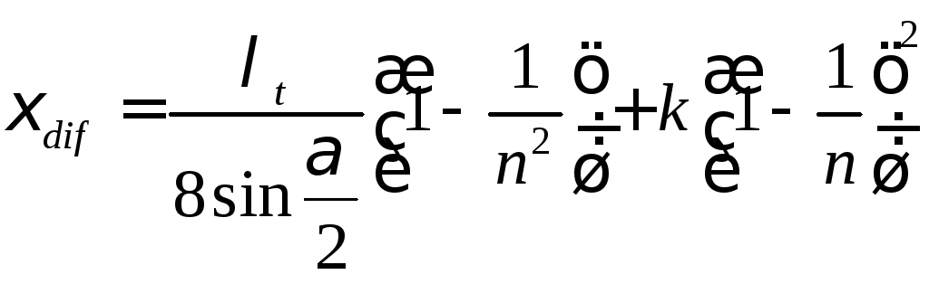(8.8)

It will be observed that depends on the angle a, the frictionfactor X_t and the rate of divergence n.

It is important to establish how dependent on a. With anglea increasing for a given λ_t and n, the first term in Eq. (8.8), which is due to friction, decreases, as the cone is shorter, and the second, which is due to turbulence and separation, increases.

When angle a decreases eddy formation is less, but friction is greater, as for a given rate of divergence n the diffuser is longer and the friction surface increases accordingly.

The function is minimum at some optimum value ofa (Fig. 64).

The values of the cone angle can be found approximately from Eq.(8.8), replacing by 1/2 sin a, as follows: differentiate Eq. (8.8)with respect to a taking into account Eq. (8.6), equate it to

zero and solve for a:

Substituting into this for­mula friction factors of the order X_t = 0.015-0.025 and a rate of divergence of the order n = 2-4, we obtain a mean opti­mum cone angle of about 6°, which is confirmed by experimental data.

In real solutions, in order to reduce the diffuser length for a given value of n, the cone angle is made somewhat larger, viz., α = 7-9°. The value of a for square diffusers is commonly taken the same.

For rectangular diffusers diverging in one plane (flat diffusers) the optimum divergence angle is greater than for conical or square diffusers, amounting to 10-12°.

If space limitations make it impossible to use divergence angles in the optimum range, at α > 15-25°, specially designed diffusers

should be used which ensure a constant pressure gradient along the centre line (dp/dx = const). Such a curved diffuser is shown schemat­ically in Fig. 65.

The reduction in energy loss in such diffuses, as compared with straight cones, is the greater the larger the соде angle a, reaching 40 per cent at a of the order of 40-60°. Furthermore, in a curved diffuser the flow is more stable.

Good results are also obtained by using stepped diffusers, consist­ing of an ordinary optimum-angle diffuser followed by an abrupt expansion (Fig. 66). The latter does not cause high energy losses as the velocity drops considerably by the time the flow reaches the en­largement. The total resistance of such a diffuser is much less than that of an ordinary diffuser of the same length and rate of divergence.