16. Bernoulli's equation for real flow

In going over from adifferential streain tube of an ideal liquid to real flow, i. e., a stream of visctius fluid having finite dimensions and constrained by walls, it is necessary to take into account: first, nonuniform velocity distribution across the sections and, second, energy (head) losses, both of whicb are due to viscosity.

When a viscous liquid moves along a solid surface, say in a pipe, the flow is retarded due to viscosity and molecular adhesion between the liquid and the walls. The velocity therefore, is greatest along the centre line of the stream. The closer to the walls the less the speed, down to zero. The result is a velocity profile like the one shown in Fig. 28.

The velocity variations mean that layers of the liquid are slipping relative to one another as a result of which tangential shearing strains, or friction stresses, appear. Furthermore, in a viscous liquid the particles often move erratically in swirls and eddies. This re­sults in loss of energy, therefore the total energy, or total head, of a viscous stream is not constant as in the case of an ideal liquid. It is gradually dissipated in overcoming the resistances and drops along the stream.

Owing to nonuniform velocity distribution the notions of mean velocity v_m across a section (see Sec. 14) and mean specific energy at that section must be introduced.

Before investigating Bernoulli's equation for a real liquid we shall assume that the basic hydrostatic law holds good for the cross-sections considered in the form of Eq. (2.3), i. e., that the piezometric head is constant for a given section:

(across the section).

Thereby we assume that stream tubes in a moving liquid exert the same transverse pressure on each other as in a motionless liquid. This is actually the case, and it can be proved theoretically for the case of parallel streamlines across a given section, which is the kind of cross-sections we shall consider.

Let us introduce the concept of power of a flow. Power is defined as the total energy of a flow transferred through a given section per unit time. As the energy of the fluid particles varies across a section, let us first express the elementary power, i. e., the power of a dif­ferential stream tube, in terms of the total specific energy of the fluid at a given point and the differential weight rate of discharge.

We have

The power of the whole stream is found by integrating the fore­going expression over the whole of area S:

or, taking into account the assumption made,

The mean total specific energy of the fluid across the section is found by dividing the total power of the stream by the weight rate of discharge. Using the expression (4.4), we have

* It should be borne in mind that the only real pressure in this equation is the static pressure p. The other two terms, zγ and , however, can easily be expressed in terms of pressure p, which is why they are also called "pressures”.

Multiplying and dividing the last term by we obtain

(4.14)

where a is a dimensionless coefficient introduced to take account of nonuniform velocity distribution and equal to

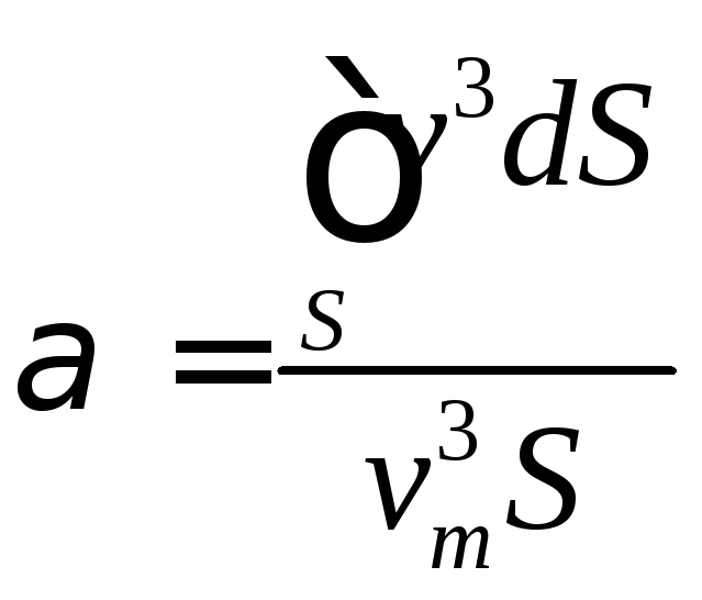(4.15)

Multiplying the numerator and denominator of this expression by , we find that the coefficient a represents the ratio of the actual kinetic energy of the stream at a given section to its kinetic energy if the velocity distribution was uniform across the section. For the commonly observed velocity distribution (Fig.28), a is always great­er than unity*, being unity when the velocity profile is a straight line.

Consider two cross-sections of a real stream, denoting the mean total head at those sections by and respectively. Then,

(4.16)

where 2/г = total loss of energy (or head) along the stream between the two sections.

Applying Eq. (4.14), the foregoing equation can be rewritten as follows:

(4.16')

This is Bernoulli's equation for real flow. It differs from the equa­tion for a differential stream tube in an ideal liquid by the term rep­resenting the loss of energy (head) and the coefficient which takes into account the nonuniform velocity distribution. Furthermore, the equation contains the mean velocities across the respective sec­tions.

Graphically this equation can be represented by a diagram like the one drawn for an ideal fluid, but taking into account the head losses. The latter increase steadily along the flow (Fig. 29).

Whereas Bernoulli's equation for an ideal fluid stream tube is an expression of the law of conservation of mechanical energy, for real flow it represents an energy-balance equation taking losses into account. The energy dissipated by the flow does not vanish, of course. It changes into.another, form of energy, heat, which raises the tem­perature of the liquid.

* This can be proved by expressing the velocity v in Eq. (4.15) as a sum , dividing the integral into four integrals and analysing the nu­merical value of each.

The drop in the mean value of the total energy between any two points of a stream referred to unit length is called the energy gradient. The change in,the potential energy of a fluid referred to unit length is called the hydraulic gradient. In a pipe of uniform diameter with a constant velocity profile the two gradients are apparently the same.