John Wiley & Sons - 2004 - Analysis of Genes and Genomes

318 POST-GENOME ANALYSIS 10

Amplify by PCR using gene specific primers

Spot PCR products onto polylysine coated glass slide

Dry DNA onto the slide Fix by UV crosslinking Denature DNA to make single-stranded

Figure 10.2. The construction of a DNA microarray. PCR products representing individual genes, parts of genes or other DNA are spotted onto a glass slide, and then fixed into position. The resulting single-stranded DNA can then act as a binding point for complementary, labelled, DNA sequences

developed in the laboratory of Patrick Brown at Stanford University, and that sold commercially by the company Affymetrix . The Affymetrix chips contain chemically synthesized single-stranded DNA oligonucleotides ( 25 bases in length) that are attached to a quartz surface using photolabile agents and photolithographic techniques similar to those used in the production of silicon microchips. This process results can result in as many as 500 000 individual DNA molecules being placed precisely within a 1.28 cm2 chip. The Stanford

chips are constructed by robotic spotting of DNA fragments, derived from the PCR amplification of entire genes, onto precise points of a glass slide. In the case of the yeast genome 6116 separate PCR reactions are performed to amplify every individual gene. These PCR products are then spotted onto a glass slide measuring approximately 2 cm2. Each PCR product is spotted onto a precise location. Consequently, the sequence of the DNA at any individual spot is known. Once spotted onto the slide, the DNA is dried by heating to 100 ◦C for 2 s, fixed by UV cross-linking, and then denatured (95 ◦C, 2 min) to make the DNA single stranded.

The prepared chips are then used as templates for the binding of labelled cDNA fragments. cDNA fragments are prepared as indicated in Figure 10.3. RNA samples from two related sets of cells are isolated. The cells generally have to be related to each other so that the majority of genes that they express will be similar. The cells have, however, been either grown under different conditions, or derived from, say, a normal and cancerous version of the same tissue. Single strands of cDNA are produced using reverse transcriptase from an oligo(dT) primer. The synthesis of cDNA is carried out in the presence of three normal deoxynucleotide triphosphates and a single fluorescently labelled deoxynucleotide triphosphate. One of the cDNA samples is produced using a green fluorescent label (nucleotide labelled with Cy3), while the other is produced using a red fluorescent dye (nucleotide labelled with Cy5). Consequently, the cDNA isolated from each different cell types will bear a different fluorescent marker. The cDNA samples are then mixed in equal quantities and allowed to hybridize to the microarray chip. The colour and intensity of each spot on the microarray is then monitored using a fluorescent scanning confocal microscope. The labels are excited using a laser, and the fluorescence at each spot detected with the microscope to give an indication of the relative amount of each RNA species within the original samples. For example, as shown in Figure 10.3, if the cells grown under condition 1 express a gene that is not expressed under condition 2, then the mixed cDNA will only contain the Cy3 labelled version of the corresponding cDNA and the complementary spot on the microarray will be labelled green. Similarly, a gene only expressed in growth condition 2 will yield a red spot on the array. Genes expressed at equal levels in both samples will give rise to both green and red labelled cDNAs that can both bind to the complementary sequence on the array. In this case a yellow spot (mixture of green and red) will be generated.

It is important that each microarray is calibrated so that the levels of mRNA from each of the samples can be accurately assessed (Bilban et al., 2002). The ratio between the green and red fluorescent signals is calculated for several array spots that contain total genomic DNA. The fluorescence detector can

320 POST-GENOME ANALYSIS 10

Mix and hybridize to microarray

Expressed only in condition 1

Expressed

in 1 and 2

Expressed only in condition 2

Figure 10.3. Identifying genes whose expression differs between two RNA samples using microarrays. (a) The RNA from cells grown in condition 1 is isolated and converted to cDNA using an oligo-dT primer that is itself labelled with a green fluorescent dye (Cy3). Similarly, RNA from cells grown in condition 2 is isolated and converted to cDNA using an oligo-dT primer labelled with a red fluorescent dye (Cy5). The cDNA samples are mixed in equal proportions and hybridized to the microarray. Viewing the microarray with a fluorescent microscope reveals a series of coloured spots. A green spot indicates that the corresponding gene is only expressed in condition 1, while a red spot indicates that a gene is only expressed in condition 2. If equal quantities of cDNA derived from cells 1 and 2 bind to the single-stranded DNA on the array, then equal amounts of the red and green dyes will bind to yield a yellow spot. (b) A microarray derived from mouse gene sequences used to screen different RNA samples for the expression of genes, courtesy of Yanxia Hao and Christopher Barker, The J. David Gladstone Institutes Genomics Core Laboratory, San Francisco

then be calibrated so these elements have a measured relative intensity ratio of 1.0. The relative intensity of green and red signals can then be used as a measure of the relative abundance of a specific mRNA in each sample.

There has been an explosion in the use of DNA microarrays to analyse gene expression on a genome-wide scale. Here we will discuss several specific examples where transcript profiling has been used to address biological problems, but the literature contains numerous others (Lockhart and Winzeler, 2000; Shoemaker and Linsley, 2002).

•Gene expression associated with metabolic changes. DNA microarrays have been used to measure the relative expression of all of genes in yeast

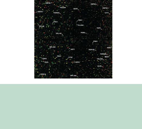
during the diauxic shift (the change from fermentative to respirative growth that occurs as glucose is depleted from the growth media) (DeRisi, Iyer and Brown, 1997). Yeast cells were harvested from a culture every two hours over a period of time and used to compare the genes being expressed in them to the initial expression pattern. From the isolated mRNA, fluorescently labelled cDNA was prepared using Cy5, while cells harvested at the first time-point (a reference sample) were labelled with Cy3. The cDNA from each of the time-points was then mixed with the reference cDNA and hybridized to a microarray chip containing each of the 6000 yeast genes. As glucose was depleted from the media, marked changes in the global pattern of gene expression were observed (Figure 10.4). Approximately 30 per cent of the genes within the genome showed altered expression levels. These genes are either upor down-regulated by at least a factor of two compared to the starting material. The metabolic shift during which glucose is depleted was correlated with widespread changes in the

(a)

Figure 10.4. Microarrays to identify the flux through metabolic pathways. (a) A yeast genome microarray in which RNA from cells grown in glucose-rich medium was labelled with Cy3 (green) and RNA form cells grown in glucose-depleted medium was labelled with Cy5 (red). (b) Metabolic reprogramming during the diauxic shift. Genes encoding the enzymes shown in red increase by the factor shown during the diauxic shift, while those in green decrease. The red arrows indicate steps in the metabolic pathway whose genes are strongly induced upon glucose depletion. These figures were kindly provided by Joe DeRisi (UC San Francisco) and are reprinted with permission from DeRisi, Iyer and Brown (1997). Copyright 1997 American Association for the Advancement of Science

9.1PGM2

PGM1

5.8HXK1

Figure 10.4. (continued)

expression of genes involved in many fundamental cellular processes, e.g. carbon metabolism, protein synthesis and carbohydrate storage. However,50 per cent of differentially expressed genes identified by the microarray analysis had no previously characterized function.

•Expression differences between normal and cancerous cells. DNA microarrays have been used extensively to characterize genes that are differentially expressed in cancer cells. For example, the analysis of 5500 genes

324 POST-GENOME ANALYSIS 10

•Defining cell type. Stem cells, which we will discuss in greater detail in Chapter 13, differ from most other cells within mammals in that they have the capacity to both self-renew and can, given the appropriate signals, differentiate into a variety of distinct cell types. Three of the best characterized types of stem cell have been isolated from embryonic, neural and hematopoietic tissue (Blau, Brazelton and Weimann, 2001). Using microarrays, transcript profiling of these different types of stem cell has revealed the presence of approximately 200 genes that are expressed within different stem cells that are not expressed within differentiated cells (Ivanova et al., 2002; Ramalho-Santos et al., 2002). These genes may describe a unique genetic programme that allows the cells to function as stem cells.

DNA microarrays offer the opportunity to analyse the expression of many thousands of genes in a single experiment. They do, however, suffer from a number of deficiencies. For example, like all the experiments we have discussed that rely on nucleic acid hybridization, the cross-hybridization of highly similar sequences can prove problematical. The data obtained from the microarray experiment must therefore be confirmed by more traditional gene expression analysis experiments. Additionally, the overall sensitivity of the microarray experiment is not high. Changes in the expression of a gene can only usually be detected if changes by a factor of two or more occur. Subtle changes in expression, which may have vital physiological roles, may go undetected during microarray analysis. Of course, the production of some proteins is not regulated at the level of transcription. For example, the gene encoding the yeast transcriptional activator Gcn4p is transcribed constitutively, but the production of protein is controlled at the level of translation in response to amino acid starvation (Hinnebusch, 1997). Finally, the sheer amount of data generated by microarrays has led to difficulties in how this information is analysed, and stored in an accessible format. The efforts of many bioinformaticians are currently aimed at presenting such data in a format that is usable by biologists. Databases of publicly available raw and normalized microarray data (e.g. http://www.dnachip.org) allow the inspection of microarrays to see how your favourite gene is regulated under particular conditions.

10.1.3ChIPs with Everything

A natural extension of seeing which genes are expressed under particular conditions is to ask what are the transcription factors that control the expression of the regulated genes. Traditional biochemical methods (e.g. DNA footprinting and gel retardation) have been used to identify the regions of DNA to which a

transcription factor can bind. Inferences can then be made as to which genes are controlled by the transcription factor by looking for particular DNA binding sites within the promoters of genes. This approach has been very successful in identifying potential target genes, but suffers from the fact that many transcription factors bind to relatively ill defined DNA sites that occur far more frequently within the genome than the number of genes actually regulated by the protein. What is required is a way of identifying genuine DNA binding sites for particular transcription factors based on the sequences that they actually bind within the cell. Chromatin immunoprecipitation (ChIP) is a method designed to do just that (Strahl-Bolsinger et al., 1997). Growing cells are treated with formaldehyde, a cross-linking agent, to attach covalently proteins and DNA that are in close physical proximity with each other (Figure 10.6). The cells are then broken open and the DNA sheared by sonication to generate fragments of about 500 bp in length. This process will not disrupt the formaldehyde crosslinks, so proteins should remain attached to their cognate DNA binding sites. DNA fragments bound by individual proteins are then separated from the rest through the interaction of the protein with a specific antibody raised against it. The antibody–antigen complexes may be precipitated using beads that will specifically bind to the antibodies. Heating the immunoprecipitated samples to 65 ◦C for 12–18 h results in the reversal of the formaldehyde cross-links and consequent release of the DNA from the DNA–protein complexes. The presence of individual promoter sequences in the immunoprecipitated fraction can then be assayed using PCR. Specific primers to the promoters of individual genes are then used to detect the presence of that particular DNA sequence in the antibody associated DNA fraction (Hecht and Grunstein, 1999). A positive PCR reaction is an indication that one or more binding sites for the protein against which the antibody was raised are present within the promoter being tested. Through careful design of the PCR, the relative occupancy of individual DNA binding sites within a promoter can be determined. Additionally, changes in promoter occupancy associated with altered cellular conditions can be observed as changes in the intensity of the PCR product.

ChIP analysis is a powerful way to identify DNA binding sites for proteins at known promoters. However, the technique is even more useful when combined with microarray chips to identify protein binding sites on a genome-wide scale. As shown in Figure 10.6, DNA fragments cross-linked to a protein of interest are enriched by immunoprecipitation with a specific antibody. After the reversal of the cross-links, the enriched DNA is amplified and labelled with a fluorescent dye (Cy5). A sample of DNA not enriched by immunoprecipitation is labelled with a different fluorophore (Cy3), and a mixture of the enriched and un-enriched pools of labelled DNA are hybridized to a microarray containing

326 POST-GENOME ANALYSIS 10

Crosslink

Break open cells and sonicate DNA

Add antibody

Purify antibody complexes

Reverse crosslinks, add specific primers

PCR

Gel of PCR products

Figure 10.6. Chromatin immunoprecipitation (ChIP) to identify the occupancy of specific DNA binding sites within genomic DNA. See the text for details

all intergenic and promoter DNA sequences. This was first used to identify the genomic binding sites of two yeast transcription factors, Gal4p and Ste12p (Ren et al., 2000). Three previously unidentified gene targets for the exceptionally well characterized Gal4p were identified using this ChIP-on-chip analysis. Subsequently, the binding sites for (and by inference the genes regulated by) 106 yeast transcriptional activators have been identified (Lee et al., 2002). A

number of additional experiments have extended the analysis of transcription factor binding sites to insect (Berman et al., 2002) and human cells (Weinmann et al., 2002). Perhaps unexpectedly, analysis of this type has shown that many genes in higher eukaryotes that are co-ordinately expressed from the same transcription factor binding sites are located in clusters next to each other on the genome (Roy et al., 2002). The significance of this finding is not completely understood, but may suggest a higher order of gene organization within the genome that may be involved in the control of their expression.

10.2Protein Function on a Genome-wide Scale

Knowing what genes are expressed in a cell at any particular time is informative, but it does not give information as to the function of particular gene products. Methods have therefore been devised to analyse protein function at a genomewide level. These have relied on either disrupting individual genes so that individual proteins are eliminated from the cell, or mapping the interactions between sets of proteins.

10.3Knock-out Analysis

Despite decades of extensive genetic analysis, approximately one-third of the6000 genes in the yeast genome have no ascribed function. The elimination of a single gene product from the genome can yield important clues as to the function of that gene through the phenotypic analysis of the resulting mutant. For many years, researchers have been able to knock out individual genes in yeast cells using homologous recombination (Rothstein, 1983). This process, which occurs at high frequency in yeast, replaces a target gene with one possessing a selectable phenotype (Figure 10.7). A linear DNA fragment bearing the selectable gene is constructed such that it is surrounded at its 5 - and 3 -ends by at least 50 bp of sequence derived from the gene to be disrupted. Transformation of yeast with this DNA fragment, which cannot independently replicate, results in its integration into the genome at the precise location of the homologous sequences. Consequently, the target gene, originally located between the homologous sequences, will be eliminated and replaced by the selectable gene. The elucidation of the entire yeast genome sequence has led to the systematic disruption of every gene (Winzeler et al., 1999). The method used involves a PCR based gene strategy to generate deletion mutants of each gene from its start codon to its stop codon. During the deletion process, each target gene is replaced with a KanMX cassette (Wach et al., 1994). This