Broadband Packet Switching Technologies

Fig. 2.20 The cell loss probability for completely shared buffering as a function of the buffer size per output, b, and the switch size N, for offered loads Ža. p s 0.8 and Žb. p s 0.9.

46 BASICS OF PACKET SWITCHING

are only interested in the region of low cell loss probability Že.g., less than 10y6 ., in which this approximation is still good.

When N is finite, Ai, which is the number of cell arrivals destined for output i in the steady state, is not independent of A j Ž j i.. This is because at most N cells arrive at the switch, and a large number of cells arriving for one output implies a small number for the remaining outputs. As N goes to infinity, however, Ai becomes an independent Poisson random variable Žwith mean value p.. Then Qi, which is the number of cells in the buffer that are destined for output i in the steady state, also becomes independent of Qj Ž j i.. We will use the Poisson and independence assumptions for finite N. These approximations are good for N G 16.

Therefore we model the steady-state distribution of ÝiNs1 Qi, the number of cells in the buffer, as the N-fold convolution of N MrDr1 queues. With the assumption of an infinite buffer size, we then approximate the cell loss probability by the overflow probability PrwÝiNs1 Qi G Nbx. Figure 2.20Ža. and Žb. show the numerical results.

REFERENCES

1.X. Chen and J. F. Hayes, ‘‘Call scheduling in multicast packet switching,’’ Proc. IEEE ICC ’92, pp. 895 899, 1992.

2.I. Cidon et al., ‘‘Real-time packet switching: a performance analysis,’’ IEEE J. Select. Areas Commun., vol. 6, no. 9, pp. 1576 1586, Dec. 1988.

3.FORE systems, Inc., ‘‘White paper: ATM switching architecture,’’ Nov. 1993.

4.J. N. Giacopelli, J. J. Hickey, W. S. Marcus, W. D. Sincoskie, and M. Littlewood, ‘‘Sunshine: a high-performance self-routing broadband packet switch architecture,’’ IEEE J. Select. Areas Commun., vol. 9, no. 8, pp. 1289 1298, Oct. 1991.

5.J. Hui and E. Arthurs, ‘‘A broadband packet switch for integrated transport,’’ IEEE J. Select. Areas Commun., vol. 5, no. 8, pp. 1264 1273, Oct. 1987.

6.A. Huang and S. Knauer, ‘‘STARLITE: a wideband digital switch,’’ Proc. IEEE GLOBECOM ’84, pp. 121 125, Dec. 1984.

7.M. J. Karol, M. G. Hluchyj, and S. P. Morgan, ‘‘Input Versus Output Queueing on a Space Division Packet Switch,’’ IEEE Trans. Commun., vol. COM-35, No. 12, Dec. 1987.

8.T. Kozaki, N. Endo, Y. Sakurai, O. Matsubara, M. Mizukami, and K. Asano, ‘‘32 32 shared buffer type ATM switch VLSI’s for B-ISDN’s,’’ IEEE J. Select. Areas Commun., vol. 9, no. 8, pp. 1239 1247, Oct. 1991.

9.S. C. Liew and T. T. Lee, ‘‘ N log N dual shuffle-exchange network with error-cor- recting routing,’’ Proc. IEEE ICC ’92, Chicago, vol. 1, pp. 1173 1193, Jun. 1992.

10.P. Newman, ‘‘ATM switch design for private networks,’’ Issues in Broadband Networking, 2.1, Jan. 1992.

11.S. Nojima, E. Tsutsui, H. Fukuda, and M. Hashimoto, ‘‘Integrated services packet network using bus-matrix switch,’’ IEEE J. Select. Areas Commun., vol. 5, no. 10, pp. 1284 1292, Oct. 1987.

REFERENCES 47

12.Y. Shobatake, M. Motoyama, E. Shobatake, T. Kamitake, S. Shimizu, M. Noda, and K. Sakaue, ‘‘A one-chip scalable 8 8 ATM switch LSI employing shared buffer architecture,’’ IEEE J. Select. Areas Commun., vol. 9, no. 8, pp. 1248 1254, Oct. 1991.

13.H. Suzuki, H. Nagano, T. Suzuki, T. Takeuchi, and S. Iwasaki, ‘‘Output-buffer switch architecture for asynchronous transfer mode,’’ Proc. IEEE ICC ’89, pp. 99 103, Jun. 1989.

14.F. A. Tobagi, T. K. Kwok, and F. M. Chiussi, ‘‘Architecture, performance and implementation of the tandem banyan fast packet switch,’’ IEEE J. Select. Areas Commun., vol. 9, no. 8, pp. 1173 1193, Oct. 1991.

15.Y. S. Yeh, M. G. Hluchyj, and A. S. Acampora, ‘‘The knockout switch: a simple, modular architecture for high-performance switching,’’ IEEE J. Select. Areas Commun., vol. 5, no. 8, pp. 1274 1283, Oct. 1987.

Broadband Packet Switching Technologies: A Practical Guide to ATM Switches and IP Routers

H. Jonathan Chao, Cheuk H. Lam, Eiji Oki

Copyright 2001 John Wiley & Sons, Inc. ISBNs: 0-471-00454-5 ŽHardback.; 0-471-22440-5 ŽElectronic.

CHAPTER 3

INPUT-BUFFERED SWITCHES

When high-speed packet switches were constructed for the first time, they used either internal shared buffer or input buffer and suffered the problem of throughput limitation. As a result, most early-date research has focused on the output buffering architecture. Since the initial demand of switch capacity is at the range of a few to 10 20 Gbitrs, output buffered switches seem to be a good choice for their high delay throughput performance and memory utilization Žfor shared-memory switches.. In the first few years of deploying ATM switches, output-buffered switches Žincluding shared-memory switches. dominated the market. However, as the demand for large-capacity switches increases rapidly Žeither line rates or the switch port number increases., the speed requirement for the memory must increase accordingly. This limits the capacity of output-buffered switches. Therefore, in order to build larger-scale and higher-speed switches, people have focused on input-buffered or combined input output-buffered switches with advanced scheduling and routing techniques, which are the main subjects of this chapter.

Input-buffered switches have two problems: Ž1. throughput limitation due to the head-of-line ŽHOL. blocking and Ž2. the need of arbitrating cells due to output port contention. The first problem can be circumvented by moderately increasing the switch fabric’s operation speed or the number of routing paths to each output port Ži.e., allowing multiple cells to arrive at the output port in the same time slot.. The second problem is resolved by novel, fast arbitration schemes that will be described in this chapter. According to Moore’s law, memory density doubles every 18 months. But the memory speed increases at a much slower rate. For instance, the memory speed in 2001 is 5 ns for state-of-the-art CMOS static RAM, compared with 6 ns one

49

50 INPUT-BUFFERED SWITCHES

or two years ago. On the other hand, the speed of logic circuits increases at a higher rate than that of memory. Recently, much research has been devoted to devising fast scheduling schemes to arbitrate cells from input ports to output ports.

Here are the factors used to compare different scheduling schemes: Ž1. throughput, Ž2. delay, Ž3. fairness for cells, independent of port positions, Ž4. implementation complexity, and Ž5. scalability as the line rate or the switch size increases. Furthermore, some scheduling schemes even consider per-flow scheduling at the input ports to meet the delay throughput requirements for each flow, which of course greatly increases implementation complexity and cost. Scheduling cells on a per-flow basis at input ports is much more difficult than at output ports. For example, at an output port, cells Žor packets. can be timestamped with values based on their allocated bandwidth and transmitted in ascending order of their timestamp values. However, at an input port, scheduling cells must take output port contention into account. This makes the problem so complicated that so far no feasible scheme has been devised.

A group of researchers attempted to use input-buffered switches to emulate output-buffered switches by moderately increasing the switch fabric operation speed Že.g., to twice the input line rate. together with some scheduling scheme. Although this has been shown to be possible, its implementation complexity is still too high to be practical.

The rest of this chapter is organized as follows. Section 3.1 describes a simple switch model with input buffers Žoptional. and output buffers, and an on off traffic model for performance study. Section 3.2 presents several methods to improve the switch performance. The degradation is mainly caused by HOL blocking. Section 3.3 describes several schemes to resolve output port contention among the input ports. Section 3.4 shows how an input-buffered switch can emulate an output-buffered switch. Section 3.5 presents a new scheduling scheme that can achieve a delay bound for an input-buffered switch without trying to emulate an output-buffered switch.

3.1 A SIMPLE SWITCH MODEL

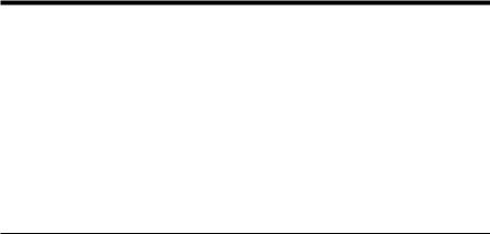
Figure 3.1 depicts a simple switch model where a packet switch is divided into several component blocks. In the middle there is a switch fabric that is responsible for transferring cells from inputs to outputs. We assume that the switch fabric is internally nonblocking and it takes a constant amount of time to deliver a group of conflict-free cells to their destination. Because of output contention, however, cells destined for the same output may not be able to be delivered at the same time, and some of them may have to be buffered at inputs. We also assume that each input link and output link has the same transmission speed to connect to the outside of the switch, but the internal switch fabric can have a higher speed to improve the performance. In this case, each output may require a buffer also.

Fig. 3.1 A switch model.

3.1.1 Head-of-Line Blocking Phenomenon

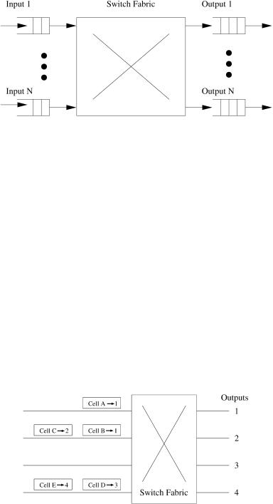
A natural way to serve cells waiting at each input is first in, first out ŽFIFO.. That is, in every time slot only the HOL cell is considered. When a HOL cell cannot be cleared due to its loss in output contention, it may block every cell behind, which may be destined for a currently idle output. In Figure 3.2, between the first two inputs, only one of the two contending HOL cells ŽA and B. can be cleared in this time slot. Although cell C Žthe second cell of the second input. is destined for a currently idle output, it cannot be cleared, because it is blocked by the HOL cell Žcell B.. This phenomenon is called HOL blocking, as described in Section 2.3.1. In this case, the inefficiency can be alleviated if the FIFO restriction is relaxed. For example, both cell A and cell C may be selected to go while cell B remains on the line until the next time slot. Scheduling methods to improve switch efficiency are discussed in Section 3.2.2.

However, no scheduling scheme can improve the case at the last input where only one of the two cells can be cleared in a time slot although each of them is destined for a distinct free output. Increasing internal bandwidth is the only way to improve this situation, and it is discussed in Section 3.2.1.

Fig. 3.2 Head-of-line blocking.

52 INPUT-BUFFERED SWITCHES

3.1.2 Traffic Models and Related Throughput Results

This subsection briefly describes how the FIFO service discipline limits the throughput under some different traffic models. Detailed analytical results are described in Section 2.3.1.

3.1.2.1Bernoulli Arrival Process and Random Traffic Cells arrive at each input in a slot-by-slot manner. Under Bernoulli arrival process, the probability that there is a cell arriving in each time slot is identical and is independent of any other slot. This probability is referred as the offered load of the input. If each cell is equally likely to be destined for any output, the traffic becomes uniformly distributed over the switch.

Consider the FIFO service discipline at each input. Only the HOL cells contend for access to the switch outputs. If every cell is destined for a different output, the switch fabric allows each to pass through to its output. If

k HOL cells are destined for the same output, one is allowed to pass through the switch, and the other k y 1 must wait until the next time slot. While one cell is waiting its turn for access to an output, other cells may be queued behind it and blocked from possibly reaching idle outputs. A Markov model can be established to evaluate the saturated throughput when N is small.1 When N is large, the slot-by-slot number of HOL cells destined for a

particular output becomes a Poisson process. As described in Section 2.3.1, the HOL blocking limits the maximum throughput to 0.586 when N ™ .

3.1.2.2On–Off Model and Bursty Traffic In the bursty traffic model, each input alternates between active and idle periods of geometrically distributed duration. During an active period, cells destined for the same output arrive continuously in consecutive time slots. The probability that an active or an idle period will end at a time slot is fixed. Denote p and q as the probabilities for an active and for an idle period, respectively. The duration of an active or an idle period is geometrically distributed as expressed in the following:

Note that it is assumed that there is at least one cell in an active period. An active period is usually called a burst. The mean burst length is then given by

1 Consider the state as one of the different destination combinations among the HOL cells.

and the offered load is the portion of time that a time slot is active:

Under bursty traffic, it has been shown that, when N is large, the throughput of an input-buffered switch is between 0.5 and 0.586, depending on the burstiness w19x.

3.2 METHODS FOR IMPROVING PERFORMANCE

The throughput limitation of an input-buffered switch is primarily due to the bandwidth constraint and the inefficiency of scheduling cells from inputs to outputs. To improve the throughput performance, we can either develop more efficient scheduling methods or simply increase the internal capacity.

3.2.1Increasing Internal Capacity

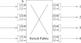
3.2.1.1Multiline (Input Smoothing) Figure 3.3 illustrates an arrange-

ment where the cells within a frame of b time slots at each of the N inputs are simultaneously launched into a switch fabric of size Nb Nb w13, 9x. At most Nb cells enter the fabric, of which b can be simultaneously received at each output. In this architecture, the out-of-sequence problem may occur at any output buffer. Although intellectually interesting, input smoothing does not seem to have much practical value.

3.2.1.2Speedup A speedup factor of c means that the switch fabric runs c times as fast as the input and output ports w20, 12x. A time slot is further

divided into c cycles, and cells are transferred from inputs to outputs in every cycle. Each input Žoutput. can transmit Žaccept. c cells in a time slot.

Fig. 3.3 Input smoothing.

54 INPUT-BUFFERED SWITCHES

Simulation studies show that a speedup factor of 2 yields 100% throughput w20, 12x.

There is another meaning when people talk about ‘‘speedup’’ in the literature. At most one cell can be transferred from an input in a time slot, but during the same period of time an output can accept up to c cells w27, 6, 28x. In bursty traffic mode, a factor of 2 only achieves 82.8% to 88.5% throughput, depending on the degree of input traffic correlation Žburstiness. w19x.

3.2.1.3Parallel Switch The parallel switch consists of K identical switch planes w21x. Each switch plane has its own input buffer and shares output buffers with other planes. The parallel switch with K s 2 achieves the maximum throughput of 1.0. This is because the maximum throughput of each switch plane is more than 0.586 for arbitrary switch size N. Since each input port distributes cells to different switch planes, the cell sequence is out of order at the output port. This type of parallel switch requires timestamps, and cell sequence regeneration at the output buffers. In addition, the hardware resources needed to implement the switch are K times as much as for a single switch plane.

3.2.2Increasing Scheduling Efficiency

3.2.2.1Window-Based Lookahead Selection Throughput can be increased by relaxing the strict FIFO queuing discipline at input buffers. Although each input still sends at most one cell into the switch fabric per time slot, it is not necessarily the first cell in the queue. On the other hand, no more than one cell destined for the same output is allowed to pass through the switch fabric in a time slot. At the beginning of each time slot,

the first w cells in each input queue sequentially contend for access to the switch outputs. The cells at the heads of the input queues ŽHOL cells. contend first. Due to output conflict, some inputs may not be selected to transmit the HOL cells, and they send their second cells in line to contend for access to the remaining outputs that are not yet assigned to receive cells in this time slot. This contention process is repeated up to w times in each time slot. It allows the w cells in an input buffer’s window to sequentially

contend for any idle outputs until the input is selected to transmit a cell. A window size of w s 1 corresponds to input queuing with FIFO buffers.

Table 3.1 shows the maximum throughput achievable for various switch and window sizes Ž N and w, respectively.. The values were obtained by

simulation. The throughput is significantly improved on increasing the window size from w s 1 Ži.e., FIFO buffers. to w s 2, 3, and 4. Thereafter,

however, the improvement diminishes, and input queuing with even an infinite window Žw s . does not attain the optimal delay throughput performance of output queuing. This is because input queuing limits each input to send at most one cell into the switch fabric per time slot, which prevents cells from reaching idle outputs.

TABLE 3.1 The Maximum Throughput Achievable with Input Queuing for Various Switch Sizes N and Window Sizes w

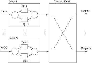
Fig. 3.4 Virtual output queue at the input ports.

3.2.2.2 VOQ-Based Matching Another way to alleviate the HOL blocking in input-buffered switches is for every input to provide a single and separate FIFO for each output. Such a FIFO is called a virtual output queue ŽVOQ., as shown in Figure 3.4. For example, VOQi, j stores cells arriving at input port i and destined for output port j.

With virtual output queuing, an input may have cells granted access by more than one output. Since each input can transfer only one cell in a time slot, the others have to wait, and their corresponding outputs will be idle. This inefficiency can be alleviated if the algorithm runs iteratively. In more intelligent schemes, matching methods can be applied to have the optimal scheduling. Three matching methods are introduced: maximal matching, maximum matching, and stable matching.