Broadband Packet Switching Technologies

Broadband Packet Switching Technologies: A Practical Guide to ATM Switches and IP Routers

H. Jonathan Chao, Cheuk H. Lam, Eiji Oki

Copyright 2001 John Wiley & Sons, Inc. ISBNs: 0-471-00454-5 ŽHardback.; 0-471-22440-5 ŽElectronic.

CHAPTER 2

BASICS OF PACKET SWITCHING

This chapter discusses the basic concepts in designing an ATM switch. An ATM switch has multiple inputroutput ports, each connecting to another port of an ATM switch or an ATM terminal. An ATM terminal can be a personal computer, a workstation, or any other equipment that has an ATM network interface card ŽNIC.. The physical layer of interconnecting ATM switches or ATM terminals can be SONET Žsuch as OC-3c, OC-12c, OC-48, or OC-192. or others Žsuch as T1 or T3.. Physical layer signals are first terminated and cells are extracted for further processing, such as table lookup, buffering, and switching. Cells from different places arrive at the input ports of the ATM switch. They are delivered to different output ports according to their labels, merged with other cell streams, and put into physical transmission frames. Due to the contention of multiple cells from different input ports destined for the same output port simultaneously, some cells must be buffered while the other cells are transmitted to the output ports. Thus, routing cells to the proper output ports and buffering them when they lose contention are the two major functions of an ATM switch.

Traditional telephone networks use circuit switching techniques to establish connections. In the circuit switching scheme, there is usually a centralized processor that determines all the connections between input and output ports. Each connection lasts on average 3 min. For an N N switch, the time required to make each connection is 180 seconds divided by N. For instance, suppose N is 1000. The connection time is 180 ms, which is quite relaxed for most of switch fabrics using current technology, such as CMOS crosspoint switch chips. However, for ATM switches, the time needed to

15

16 BASICS OF PACKET SWITCHING

configure the inputroutput connections is much more stringent, because it is based on the cell time slot. For instance, for the OC-12c interface, each cell slot time is about 700 ns. For an ATM switch with 1000 ports, the time to make the connection for each inputroutput is 700 ps, which is very challenging for existing technology. Furthermore, as the line bit rate increases Že.g., with OC-48c. and the number of the switch ports increases, the time needed for each connection is further reduced. As a result, it is too expensive to employ centralized processors for ATM switches.

Thus, for ATM switches we do not use a centralized connection processor to establish connections. Rather, a self-routing scheme is used to establish inputroutput connections in a distributed manner. In other words, the switch fabric has the ability to route cells to proper output ports, based on the physical output port addresses that are attached in the front of each cell. One switch fabric that has self-routing capability is called the banyan switch. It will be discussed in more detail in Chapter 5.

In addition to the routing function to the ATM switch, another important function is to resolve the output port contention when more than one cell is destined for the same output port at the same time. There are several contention-resolution schemes that have been proposed since the first ATM switch architecture was proposed in early 1980s Žthe original packet switch was called a high-speed packet switch; the term ATM was not used until late 1980.. One way to resolve the contention is to allow all cells that are destined for the same output port to arrive at the output port simultaneously. Since only one cell can be transmitted via the output link at a time, most cells are queued at the output port. A switch with such architecture is called an output-buffered switch. The price to pay for such scheme is the need for operating the switch fabric and the memory at the output port at a rate N times the line speed. As the line speed or the switch port number increases, this scheme can have a bottleneck. However, if one does not allow all cells to go to the same output port at the same time, some kind of scheduling scheme, called an arbitration scheme, is required to arbitrate the cells that are destined for the same output port. Cells that lose contention will need to wait at the input buffer. A switch with such architecture is called an input-buffered switch.

The way of handling output contention will affect the switch performance, complexity, and implementation cost. As a result, most research on ATM switch design is devoted to output port contention resolution. Some schemes are implemented in a centralized manner, and some in a distributed manner. The latter usually allows the switch to be scaled in both line rate and switch size, while the former is for smaller switch sizes and is usually less complex and costly.

In addition to scheduling cells at the inputs to resolve the output port contention, there is another kind of scheduling that is usually implemented at the output of the switch. It schedules cell or packet transmission according to

the allocated bandwidth to meet each connection’s delayrthroughput requirements. Cells or packets are usually timestamped with values and transmitted with an ascending order of the timestamp values. We will not discuss such scheduling in this book, but rather focus on the scheduling to resolve output port contention.

In addition to scheduling cells to meet the delay throughput requirement at the output ports, it is also required to implement buffer management at the input or output ports, depending on where the buffer is. The buffer management discards cells or packets when the buffer is full or exceeds some predetermined thresholds. The objectives of the buffer management are to meet the requirements on cell loss rate or fairness among the connections, which can have different or the same loss requirements. There is much research in this area to determine the discarding policies. Some of them will push out the cells or packets that have been stored in the buffer to meet the loss or fairness objectives, which is usually more complex than the scheme that blocks incoming cells when the buffer occupancy exceeds some thresholds. Again this book will focus on the switch fabric design and performance studies and will not discuss the subject of buffer management. However, when designing an ATM switch, we need to take into consideration the potential need for performing packet scheduling and buffer management. The fewer locations of the buffers on the data path, the less such control is required, and thus the smaller the implementation cost.

Section 2.1 presents some basic ATM switching concepts. Section 2.2 classifies ATM switch architectures. Section 2.3 describes performance of typical basic switches.

2.1 SWITCHING CONCEPTS

2.1.1 Internal Link Blocking

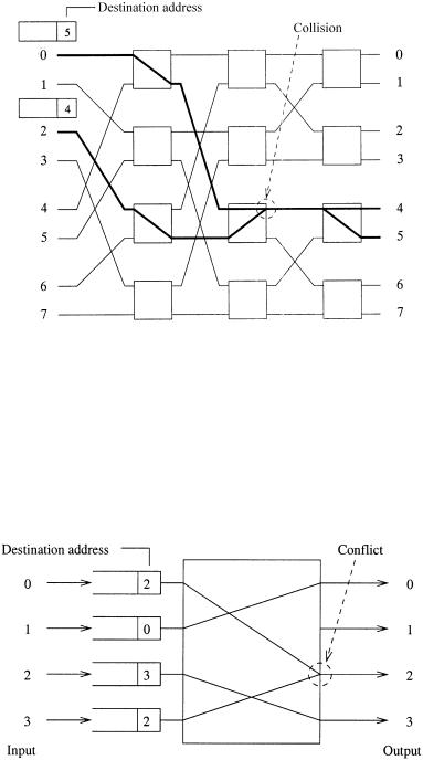
While a cell is being routed in a switch fabric, it can face a contention problem resulting from two or more cells competing for a single resource. Internal link blocking occurs when multiple cells contend for a link at the same time inside the switch fabric, as shown in Figure 2.1. This usually happens in a switch based on space-division multiplexing, where an internal physical link is shared by multiple connections among inputroutput ports. A blocking switch is a switch suffering from internal blocking. A switch that does not suffer from internal blocking is called nonblocking. In an internally buffered switch, contention is handled by placing buffers at the point of conflict. Placing internal buffers in the switch will increase the cell transfer delay and degrade the switch throughput.

18 BASICS OF PACKET SWITCHING

Fig. 2.1 Internal blocking in a delta network: two cells destined for output ports 4 and 5 collide.

2.1.2 Output Port Contention

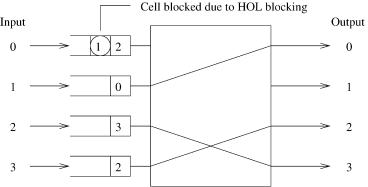
Output port contention occurs when two or more cells arrive from different input ports and are destined for the same output port, as shown in Figure 2.2. A single output port can transmit only one cell in a time slot; thus the other cells must be either discarded or buffered. In the output-buffered switches, a buffer is placed at each output to store the multiple cells destined for that output port.

Fig. 2.2 Output port contention.

2.1.3 Head-of-Line Blocking

Another way to resolve output port contention is to place a buffer in each input port, and to select only one cell for each output port among the cells destined for that output port before transmitting the cell. This type of switch is called the input-buffered switch. An arbiter decides which cells should be chosen and which cells should be rejected. This decision can be based on cell priority or timestamp, or be random. A number of arbitration mechanisms have been proposed, such as ring reservation, sort-and-arbitrate, and route- and-arbitrate. In ring reservation, the input ports are interconnected via a ring, which is used to request access to the output ports. For switches that are based on a sorting mechanism in the switch fabric, all cells requesting the same output port will appear adjacent to each other after sorting. In the route-and-arbitrate approach, cells are routed through the switch fabric and arbiters detect contention at the point of conflict.

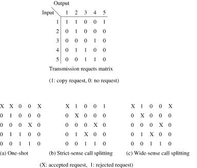
A well-known problem in a pure input-buffered switch with first-in-first- out ŽFIFO. input buffers is the head-of-line ŽHOL. blocking problem. This happens when cells are prevented from reaching a free output because of other cells that are ahead of it in the buffer and cannot be transmitted over the switch fabric. As shown in Figure 2.3, the cell behind the HOL cell at input port 0 is destined for an idle output port 1. But it is blocked by the HOL cell, which failed a transmission due to an output contention. Due to the HOL blocking, the throughput of the input buffered switch is at most 58.6% for random uniform traffic w5, 7x.

2.1.4 Multicasting

To support videoraudio conference and data broadcasting, ATM switches should have multicast and broadcast capability. Some switching fabrics achieve multicast by first replicating multiple copies of the cell and then routing each

Fig. 2.3 Head-of-line blocking.

20 BASICS OF PACKET SWITCHING

copy to their destination output ports. Other switches achieve multicast by utilizing the inherent broadcasting nature of the shared medium without generating any copies of ATM cells w3x. Details will be discussed later in the book.

2.1.5 Call Splitting

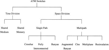
Several call scheduling disciplines have been proposed for the multicast function, such as one-shot scheduling, strict-sense call splitting, and widesense call splitting w1x. One-shot scheduling requires all the copies of the same cell to be transmitted in the same time slot. Strict-sense ŽSS. call splitting and wide-sense ŽWS. call splitting permit the transmission of the cell to be split over several time slots. For real-time applications, the delay difference among the receivers caused by call splitting should be bounded. A matrix is introduced to describe the operation of the scheduling algorithm, as shown in Figure 2.4, where each row Žcolumn. corresponds to an input line Žoutput line. of the switch. With the multicast feature each row may contain two or more 1’s rather than a single 1 in the unicast case. At each time slot only one cell can be selected from each column to establish a connection.

Fig. 2.4 Call scheduling disciplines.

2.1.5.1One-Shot Scheduling In a one-shot scheduling policy, all copies of the same cell must be switched successfully in one time slot. If even one copy loses the contention for an output port, the original cell waiting in the

input queue must try again in the next time slot. It is obvious that this strategy favors cells with fewer copies Ži.e., favors calls with fewer recipients., and more often blocks multicast cells with more copies.

2.1.5.2Strict-Sense Call Splitting In one-shot discipline, if only one copy loses contention, the original cell Žall its copies. must retry in the next time slot, thus degrading the switch’s throughput. This drawback suggests transmitting copies of the multicast cell independently. In SS call splitting, at most one copy from the same cell can be transmitted in a time slot. That is, a multicast cell must wait in the input queue for several time slots until all of its copies have been transmitted. If a multicast cell has K copies to transmit, it needs at least K time slots to transmit them. Statistically this algorithm results in a low throughput when the switch is underloaded during light traffic, since the algorithm does not change dynamically with the traffic pattern.

2.1.5.3Wide-Sense Call Splitting The case of light traffic should be considered when only one active input line has a multicast cell to be transmitted and all output ports are free. In this case, SS call splitting only allows one cell to be transmitted per time slot, resulting in a low utilization. WS call splitting was proposed to allow more than one copy from the same multicast cell to gain access to output ports simultaneously as long as these output ports are free.

It is clear that one-shot discipline has the lowest throughput performance among all three algorithms; however, it is easiest to implement. SS call splitting performs better than one-shot in the heavy traffic case, but it seems rigid in the light traffic case and results in a low utilization. WS call splitting has the advantage of the full use of output trunks, allowing the multicast cell to use all free output ports, which results in a higher throughput.

2.2SWITCH ARCHITECTURE CLASSIFICATION

ATM switches can be classified based on their switching techniques into two groups: time-di®ision switching ŽTDS. and space-di®ision switching ŽSDS.. TDS is further divided into shared-memory type and shared-medium type. SDS is further divided into single-path switches and multiple-path switches, which are in turn further divided into several other types, as illustrated in Figure 2.5. In this section, we briefly describe the operation, advantages, disadvantages, and limitations inherent in each type of switch.

22 BASICS OF PACKET SWITCHING

Fig. 2.5 Classification of ATM switching architectures.

2.2.1 Time-Division Switching

In TDS, there is a single internal communication structure, which is shared by all cells traveling from input ports to output ports through the switch. The internal communication structure can be a bus, a ring, or a memory. The main disadvantage of this technique is its strict capacity limitation of the internal communication structure. However, this class of switch provides an advantage in that, since every cell flows across the single communication structure, it can easily be extended to support multicastrbroadcast operations.

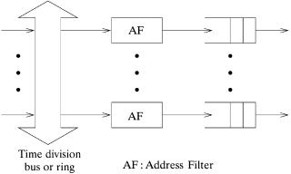
2.2.1.1 Shared-Medium Switch In a shared-medium switch, cells arriving at input ports are time-division multiplexed into a common high-speed medium, such as a bus or a ring, of bandwidth equal to N times the input line rate. The throughput of this shared medium determines the capacity of the entire switch. As shown in Figure 2.6, each output line is connected to the shared high-speed medium via an interface consisting of an address filter ŽAF. and an output FIFO buffer. The AF examines the header part of the incoming cells, and then accepts only the cells destined for itself. This decentralized approach has an advantage in that each output port can operate independently and can be built separately. However, more hardware logic and more buffers are required to provide the separate interface for each output port.

A time slot is divided into N mini-slots. During each mini-slot, a cell from an input is broadcast to all output ports. This simplifies the multicasting process. A bit map of output ports with each bit indicating if the cell is routed to that output port can be attached to the front of the cell. Each AF will examine only the corresponding bit to decide if the cell should be stored

Fig. 2.6 Shared-medium switching architecture.

in the following FIFO. One disadvantage of this structure is that the switch size N is limited by the memory speed. In particular, when all N input cells are destined for the same output port, the FIFO may not be able to store all N cells in one time slot if the switch size is too large or the input line rate is too high. Another disadvantage is the lack of memory sharing among the FIFO buffers. When an output port is temporarily congested due to high traffic loading, its FIFO buffer is filled and starts to discard cells. Meanwhile, other FIFO buffers may have plenty of space but cannot be used by the congested port. As a result, a shared-memory switch, as described below, has a better buffer utilization.

Examples of shared-medium switches are NEC’s ATOM ŽATM output buffer modular. switch w13x, IBM’s PARIS Žpacketized automated routing

integrated system. switch w2x, and Fore System’s ForeRunner ASX-100 switch w3x.

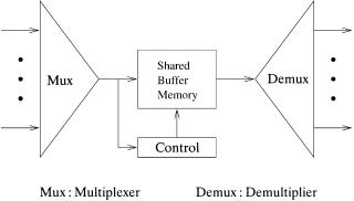
2.2.1.2 Shared-Memory Switch In a shared-memory switch, as shown in Figure 2.7, incoming cells are time-division multiplexed into a single data stream and sequentially written to the shared memory. The routing of cells is accomplished by extracting stored cells to form a single output data stream, which is in turn demultiplexed into several outgoing lines. The memory addresses for both writing incoming cells and reading out stored cells are provided by a control module according to routing information extracted from the cell headers.

The advantage of the shared-memory switch type is that it provides the best memory utilization, since all inputroutput ports share the same memory. The memory size should be adjusted accordingly to keep the cell loss rate below a chosen value. There are two different approaches in sharing

24 BASICS OF PACKET SWITCHING

Fig. 2.7 Basic architecture of shared-memory switches.

memory among the ports: complete partitioning and full sharing. In complete partitioning, the entire memory is divided into N equal parts, where N is the number of inputroutput ports, and each part is assigned to a particular output port. In full sharing, the entire memory is shared by all output ports without any reservation. Some mechanisms, such as putting an upper and a lower bound on the memory space, are needed to prevent monopolization of the memory by some output ports.

Like shared-medium switches, shared-memory switches have the disadvantage that the memory access speed limits the switch size; furthermore, the control in the shared-memory switches is more complicated. Because of its better buffering utilization, however, the shared-memory type is more popular and has more variants than the shared-medium type. Detailed discussions about those variants and their implementations are given in Chapter 4.

Examples of shared-memory switches are Toshiba’s 8 8 module on a single chip w12x and Hitachi’s 32 32 module w8x.

2.2.2 Space-Division Switching

In TDS, a single internal communication structure is shared by all input and output ports, while in SDS multiple physical paths are provided between the input and output ports. These paths operate concurrently so that multiple cells can be transmitted across the switch simultaneously. The total capacity of the switch is thus the product of the bandwidth of each path and the number of paths that can transmit cells concurrently. The total capacity of the switch is therefore theoretically unlimited. However, in practice, it is restricted by physical implementation constraints such as the device pin count, connection restrictions, and synchronization considerations.