Broadband Packet Switching Technologies

Fig. 7.22 An example of priority assignment in the concentration module.

The port priority is changed in every time slot in a RR fashion. In time slot T, ISC 1 has the highest port priority level, and ISC 3 has the lowest port priority level. In time slot T q 1, ISC 2 has the highest port priority level, and ISC 1 has the lowest port priority level, and so on. ISC 3 has a higher port priority level than ISC 1 in time slots T q 1 and T q 2.

In time slot T, all four cells in the one-cell buffers of ISC 1 pass through the CM, because they have the highest priority levels. In time slot T q 1, ISC 3 transmits two cells Ža and b. and ISC 1 transmits two cells Ž A and B.. In time slot T q 2, ISC 3 transmits one cell Žc., while ISC 1 transmits three cells ŽC, D, and E.. In time slot T q 3, ISC 1 has the highest port priority Ž0. and is able to transmit its all cells Ž F, G, H, and I .. Once they are cleared from the one-cell buffers, ISC 1 resets its sequence priority to zero.

7.6.3 Resequencing Cells

As discussed before, the routing delay in the abacus switch must be less than 424 bit times. If it is greater, there are two possibilities. First, if a cell is held up in the input buffer longer than a cell slot time, the throughput of the switch fabric will be degraded. Second, if a cell next to the HOL cell is sent to the MGN before knowing if the HOL cell is successfully transmitted to the desired output switch moduleŽs., it may be ahead of a HOL cell that did not pass through the MGN. This cell-out-of-sequence problem can be resolved with a resequencing buffer ŽRSQB. at the output port of the MGN.

For a switch size N of 1024, output group size M of 16, and group expansion ratio L of 1.25, the maximum routing delay of the single-stage abacus switch is 1043 Ži.e., N q LM y 1 as described previously.. Therefore, an arbitration cycle is at least three cell time slots. If up to three cells are allowed to transmit during each arbitration cycle, the IPC must have three one-cell buffers arranged in parallel.

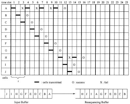
Figure 7.23 illustrates an example of the maximum extent of being out of sequence. Assume cells A to J are stored in the same input buffer in

218 THE ABACUS SWITCH

Fig. 7.23 An example of cell out of sequence with an arbitration cycle of 3 cell slots.

sequence. In time slot 1, cell A is sent to the switch fabric. It takes three time slots to know if cell A has passed through the switch fabric successfully. In time slot 2, cell B is sent to the switch fabric, and in time slot 3, cell C is sent to the switch fabric. Before the end of time slot 3, the IPC knows that cell A has failed to pass the switch fabric, so cell A will be transmitted again in time slot 4. If cell A passes through the switch fabric successfully on the fourth try, up to six cells Žcells B to G. can be ahead of cell A. The cell arrival sequence in the RSQB is shown in Figure 7.23.

For this scheme to be practical, the maximum extent of being out of sequence and the size of the RSQB should be bounded. Let us consider the worst case. If all HOL cells of N input ports are destined for the same output group and the tagged cell has the lowest port priority in time slot T, then LM highest-priority cells will be routed in time slot T. In time slot T q 1, the priority level of the tagged cell will be incremented by one, so that

Ž N y 2 LM y 1. cells whose priority levels are higher than that of the tagged cell, and so on.

The maximum extent of being out of sequence can be obtained from the following. An arbitration cycle is equal to or greater than r s

Ž N q LM y 1.r424 cell time slots. A tagged cell succeeds in at most s s NrLM tries. Therefore, in the worst case, the HOL cell passes through the switch fabric successfully in rs time slots. Denote the maximum extent of being out of sequence by t; then t s rs.

One way to implement the resequencing is to timestamp each cell with a value equal to the actual time plus t when it is sent to the switch fabric. Let us call this timestamp the due time of the cell. Cells at the RSQBs are moved to the SSM when their due times are equal to the actual time. This maintains the cell transmission sequence.

The drawbacks of this scheme are high implementation complexity of the RSQB and large cell transfer delay. Since a cell must wait in the RSQB until the actual time reaches the due time of the cell, every cell experiences at least a t cell-slot delay even if there is no contention. Table 7.4 shows the maximum extent of being out of sequence for switch sizes of 1024 and 8192. For switch size 1024, the maximum is 156 cell slots, which corresponds to 441s for the OC-3 line rate Ži.e., 156 2.83 s..

7.6.4 Complexity Comparison

This subsection compares the complexity of the above three approaches for building a large-capacity abacus switch and summarizes the results in Table 7.5. Here, the switch element in the RMs and CMs is a 2 2 crosspoint device. The number of interstage links is the number of links between the RMs and the CMs. The number of buffers is the number of ISCs. For the BMCN, the CMs have ISCs and one-cell buffers wFig. 7.21Žc.x. The second and third parts of Table 7.5 give some numerical values for a 160-Gbitrs abacus switch. Here, it is assumed that the switch size N is 1024, the input line speed is 155.52 Mbitrs, the group size M is 16, the group expansion ratio L is 1.25, and the module size n is 128.

With respect to the MMCN, there are no internal buffers and no out-of- sequence cells. Its routing delay is less than 424 bit times. But the numbers of SWEs and interstage links are the highest among the three approaches.

For the BMCN, the routing delay is no longer a concern for a large-capac- ity abacus switch. Its numbers of SWEs and interstage links are smaller than those of the MMCN. However, it may not be cost-effective when it is required to implement buffer management and cell scheduling in the inter- mediate-stage buffers to meet QoS requirements.

The last approach to resequencing out-of-sequence cells has no interstage links or internal buffers. It requires a resequencing buffer at each output

220 THE ABACUS SWITCH

TABLE 7.5 Complexity Comparison of Three Approaches for a 160-Gbitrs Abacus Switch

port. For a switch capacity of 160 Gbitrs, the delay caused by resequencing cells is at least 156 cell slot times.

7.7 ABACUS SWITCH FOR PACKET SWITCHING

The abacus switch can also handle variable-length packets. To preserve the cell1 sequence in a packet, two cell scheduling schemes are used at the input buffers. The packet interlea®ing scheme transfers all cells in a packet consecutively, while the cell interlea®ing scheme transfers cells from different inputs and reassembles them at the output.

7.7.1 Packet Interleaving

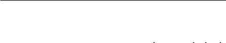
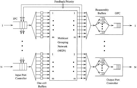
A packet switch using the packet interleaving technique is shown in Figure 7.24. The switch consists of a memoryless nonblocking multicast grouping network ŽMGN., input port controllers ŽIPCs., and output port controllers ŽOPCs.. Arriving cells are stored in an input buffer until the last cell of the packet arrives. When the last cell arrives, the packet is then eligible for transmission to output portŽs..

In the packet interleaving scheme, all cells belonging to the same packet are transferred consecutively. That is, if the first cell in the packet wins the

1 The cell discussed in this section is just a fixed-length segment of a packet and does not have to be 53 bytes like an ATM cell.

Fig. 7.24 A packet switch with packet interleaving.

output port contention for a destination among the contending input ports, all the following cells of the packet will be transferred consecutively to the destination.

A packet interleaving switch can be easily implemented by the abacus switch. Only the first cells of HOL packets can contend for output ports. The contention among the first cells of HOL packets can be resolved by properly assigning priority fields to them. The priority field of a cell has 1 q log 2 N bits. Among them, the log 2 N-bit field is used to achieve fair contention by dynamically changing its value as in the abacus switch. Prior to the contention resolution, the most significant bit ŽMSB. of the priority field is set to 1 Žlow priority.. As soon as the first cell of an HOL packet wins the contention Žknown from the feedback priorities., the MSB of the priority field of all the following cells in the same packet is asserted to 0 Žhigh priority.. As soon as the last cell of the packet is successfully sent to the output, the MSB is set to 1 for the next packet. As a result, it is ensured that cells belonging to the same packet are transferred consecutively.

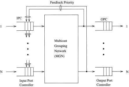
Figure 7.25 shows the average packet delay vs. offered load for a packet switch with packet interleaving. In the simulations, it is assumed that the traffic source is an on off model. The packet size is assumed to have a truncated geometric distribution with an average packet size of 10 cells and maximum packet size of 32 cells Žto accommodate the maximum Ethernet frame size.. The packet delay through the switch is defined as follows. When the last cell of a packet arrives at an input buffer, the packet is timestamped

222 THE ABACUS SWITCH

Fig. 7.25 Delay performance of a packet switch with packet interleaving.

with an arrival time. When the last cell of a packet leaves the output buffer, the packet is timestamped with a departure time. The difference between the arrival time and the departure time is defined as the packet delay. When there is no internal speedup ŽS s 1. in the switch fabric, the delay performance of the packet interleaving switch is very poor, mainly due to the HOL blocking. The delay throughput performance is improved by increasing the speedup factor S Že.g., S s 2.. Note that the input buffer’s average delay is much smaller than the output buffer’s average delay. With an internal speedup of two, the output buffer’s average delay dominates the total average delay and is very close to that of the output-buffered switch.

7.7.2 Cell Interleaving

A packet switch using a cell interleaving technique is shown in Figure 7.26. Arriving cells are stored in the input buffer until the last cell of a packet arrives. Once the last cell arrives, cells are transferred in the same way as in an ATM switch. That is, cells from different input ports can be interleaved

Fig. 7.26 A packet switch with cell interleaving.

with each other as they arrive at the output port. Cells have to carry input port numbers so that output ports can distinguish them from different packets. Therefore, each output port has N reassembly buffers, each corresponding to an input port. When the last cell of a packet arrives at the reassembly buffer, all cells belonging to the packet are moved to the output buffer for transmission to the output link. In real implementation, only pointers are moved, not the cells. This architecture is similar the one in w17x in the sense that they both use reassembly buffers at the outputs, but it is more scalable than the one in w17x.

The operation speed of the abacus switch fabric is limited to several hundred megabits per second with state-of-the-art CMOS technology. To accommodate the line rate of a few gigabits per second Že.g., Gigabit Ethernet and OC-48., we can either use a bit-slice technique or the one shown in Figure 7.26, where the high-speed cell stream is distributed to m one-cell buffers at each input port. The way of dispatching cells from the IPC to the m one-cell buffers is identical to dispatching cells from the ISC to the M one-cell buffers in Figure 7.21Žc.. The advantage of the technique in Figure 7.26 over the bit-slice technique is its smaller overhead bandwidth: the latter shrinks the cell duration while keeping the same overhead for each cell.

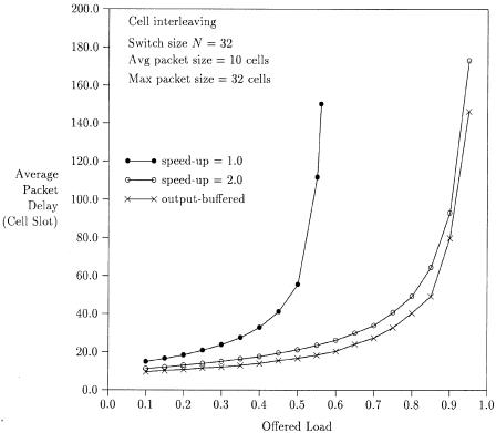
Figure 7.27 shows the average packet delay vs. offered load for a packet switch with cell interleaving. When there is no internal speedup ŽS s 1., the delay performance is poor. With an internal speedup S of two, the delay

224 THE ABACUS SWITCH

Fig. 7.27 Delay performance of a packet switch with cell interleaving.

performance is close to that of an output-buffered packet switch. By comparing the delay performance between Figure 7.25 and Figure 7.27, we can see that the average delay performance is comparable. However, we believe that the delay variation of cell interleaving will be smaller than that of packet interleaving because of its finer granularity in switching.

REFERENCES

1.B. Bingham and H. Bussey, ‘‘Reservation-based contention resolution mechanism for Batcher banyan packet switches,’’ Electron. Lett., vol. 24, no. 13, pp. 772 773, Jun. 1988.

2.C. Y. Chang, A. J. Paulraj, and T. Kailath, ‘‘A broadband packet switch architecture with input and output queueing,’’ Proc. IEEE GLOBECOM ’94, pp. 448 452, Nov. 1994.

3.H. J. Chao and N. Uzun, ‘‘An ATM routing and concentration chip for a scalable multicast ATM switch,’’ IEEE J. Solid-State Circuits, vol. 32, no. 6, pp. 816 828, Jun. 1997.

REFERENCES 225

4.H. J. Chao, B. S. Choe, J. S. Park, and N. Uzun, ‘‘Design and implementation of abacus switch: a scalable multicast ATM switch,’’ IEEE J. Select. Areas Commun., vol. 15, no. 5, pp. 830 843, Jun.1997.

5.H. J. Chao and J. S. Park, ‘‘Architecture designs of a large-capacity abacus ATM switch,’’ Proc. IEEE GLOBECOM, Nov. 1998.

6.A. Cisneros and C. A. Bracket, ‘‘A large ATM switch based on memory switches and optical star couplers,’’ IEEE J. Select. Areas Commun., vol. SAC-9, no. 8,

pp.1348 1360, Oct. 1991.

7.K. Y. Eng and M. J. Karol, ‘‘State of the art in gigabit ATM switching,’’ IEEE BSS ’95, pp. 3 20, Apr. 1995.

8.R. Handel,¨ M. N. Huber, and S. Schroder,¨ ATM Networks: Concepts, Protocols, Applications, Addison-Wesley Publishing Company, Chap. 12, 1998.

9.M. J. Karol, M. G. Hluchyj, and S. P. Morgan, ‘‘Input versus output queueing on a space-division packet switch,’’ IEEE Trans. Commun., vol. 35, pp. 1347 1356, Dec. 1987.

10.J. Hui and E. Arthurs, ‘‘A broadband packet switch for integrated transport,’’ IEEE J. Select. Areas Commun., vol. SAC-5, no. 8, pp. 1264 1273, Oct. 1987.

11.T. Kozaki, N. Endo, Y. Sakurai, O. Matsubara, M. Mizukami, and K. Asano, ‘‘32 32 shared buffer type ATM switch VLSI’s for B-ISDN’s,’’ IEEE J. Select. Areas Commun., vol. 9, no. 8, pp. 1239 1247, Oct. 1991.

12.S. C. Liew and K. W. Lu, ‘‘Comparison of buffering strategies for asymmetric packet switch modules,’’ IEEE J. Select. Areas Commun., vol. 9, no. 3, pp. 428 438, Apr. 1991.

13.Y. Oie, M. Murata, K. Kubota, and H. Miyahara, ‘‘Effect of speedup in nonblocking packet switch,’’ Proc. IEEE ICC ’89, pp. 410 415.

14.A. Pattavina, ‘‘Multichannel bandwidth allocation in a broadband packet switch,’’ IEEE J. Select. Areas Commun., vol. 6, no. 9, pp. 1489 1499, Dec. 1988.

15.A. Pattavina and G. Bruzzi, ‘‘Analysis of input and output queueing for nonblocking ATM switches,’’ IEEErACM Trans. Networking, vol. 1, no. 3, pp. 314 328, Jun. 1993.

16.E. P. Rathgeb, W. Fischer, C. Hinterberger, E. Wallmeier,and R. Wille-Fier, ‘‘The MainStreet Xpress core services node a versatile ATM switch architecture for the full service network,’’ IEEE J. Select. Areas Commun., vol. 15, no. 5,

pp.830 843, Jun.1997.

17.I. Widjaja and A. I. Elwalid, ‘‘Performance issues in VC-merge capable switches for IP over ATM networks,’’ Proc. IEEE INFOCOM ’98, pp. 372 380, Mar. 1998.

Broadband Packet Switching Technologies: A Practical Guide to ATM Switches and IP Routers

H. Jonathan Chao, Cheuk H. Lam, Eiji Oki

Copyright 2001 John Wiley & Sons, Inc. ISBNs: 0-471-00454-5 ŽHardback.; 0-471-22440-5 ŽElectronic.

CHAPTER 8

CROSSPOINT-BUFFERED SWITCHES

When more than one cell is contending for the limited link capacity inside a switch or at its outputs, buffers are provided to temporarily store the cells. Since the size of a buffer is finite, cells will be discarded when it is full. However, in previous chapters we have described several switch architectures with input buffering, output buffering Žincluding shared memory., input and output buffering, and internal buffering in a multistage structure.

This chapter describes crosspoint-buffered switches, where each crosspoint has a buffer. This switch architecture takes advantage of today’s CMOS technology, where several millions of gates and several tens of millions of bits can be implemented on the same chip. Furthermore, there can be several hundred input and output signals operating at 2 3 Gbitrs on one chip. This switch architecture does not require any increase of the internal line speed. It eliminates the HOL blocking that occurs in the input-buffered switch, at the cost of having a large amount of crosspoint-buffer memory at each crosspoint.

The remainder of this chapter is organized as follows. Section 8.1 describes a basic crosspoint-buffered switch architecture. The arbitration time among crosspoint buffers can become a bottleneck as we increase the switch size. Section 8.2 introduces a scalable distributed-arbitration ŽSDA. switch to avoid the bottleneck of the arbitration time. Section 8.3 describes an extended version of SDA to support multiple QoS classes.

227