Broadband Packet Switching Technologies

replicated cells from either MGN are aligned in time. However, the final duplicated cells at the output ports may not be aligned in time, because they may have different queueing delays in the output buffers.

6.3.2 Multicast Grouping Network

Figure 6.15 shows a modular structure for the MGN at the first or the second stage. The MGN consists of K switch modules for the first stage or M for the second stage. Each switch module contains a switch element ŽSWE. array, a number of multicast pattern maskers ŽMPMs., and an address broadcaster ŽAB.. The AB generates dummy cells that have the same destined address as the output. This enables cell switching to be done in a distributed manner and permits the SWE not to store output group address information, which simplifies the circuit of the SWE significantly and results in higher VLSI integration density. Since the structure and operation for MGN1 and MGN2 are identical, let us just describe MGN1.

Each switch module in MGN1 has N horizontal input lines and L1 M vertical routing links, where M s NrK. These routing links are shared by the cells that are destined for the same output group of a switch module. Each

Fig. 6.15 The multicast grouping network. Ž 1995 IEEE..

158 KNOCKOUT-BASED SWITCHES

input line is connected to all switch modules, allowing a cell from each input line to be broadcast to all K switch modules.

The routing information carried in front of each arriving cell is a multicast pattern, which is a bit map of all the outputs in the MGN. Each bit indicates if the cell is to be sent to the associated output group. For instance, let us consider a multicast switch with 1024 inputs and 1024 outputs and the numbers of groups in MGN1 and MGN2, K and M, both chosen to be 32. Thus, the multicast pattern in both MGN1 and MGN2 has 32 bits. For a unicast cell, the multicast pattern is basically a flattened output address Ži.e., a decoded output address. in which only one bit is set to 1 and all other 31 bits are set to 0. For a multicast cell, there are more than one bit in the multicast pattern set to 1. For instance, if a cell X is multicast to switch modules i and j, the ith and jth bits in the multicast pattern are set to 1.

The MPM performs a logic AND function for the multicast pattern with a fixed 32-bit pattern in which only the ith bit, corresponding to switch module i, is set to 1 and all other 31 bits are set to 0. So, after cell X passes through the MPM in switch module i, its multicast pattern becomes a flattened output address where only the ith bit is set to 1.

Each empty cell that is transmitted from the AB has attached to it, in front, a flattened output address with only one bit set to 1. For example, empty cells from the AB in switch module i have only the ith bit set to 1 in their flattened address. Cells from horizontal inputs will be properly routed to different switch modules based on the result of matching their multicast patterns with empty cells’ flattened addresses. For cell X, since its ith and jth bits in the multicast pattern are both set to 1, it matches with the flattened addresses of empty cells from the ABs in switch modules i and j. Thus, cell X will be routed to the output of these two switch modules.

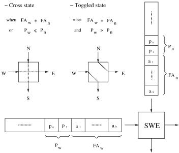
The SWE has two states, cross state and toggled state, as shown in Figure 6.16. The state of the SWE depends on the comparison result of the flattened addresses and the priority fields in cell headers. The priority is used for cell contention resolution. Normally, the SWE is at cross state, i.e., cells from the north side are routed to the south side, and cells from the west side are routed to the east side. When the flattened address of the cell from the west ŽFA w . is matched with the flattened address of the cell from the north ŽFA n., and when the west’s priority level Ž Pw . is higher than the north’s Ž Pn., the SWE’s state is toggled: The cell from the west side is routed to the south side, and the cell from the north is routed to the east. In other words, any unmatched or lower-priority Žincluding the same priority. cells from the west side are always routed to the east side. Each SWE introduces a 1-bit delay as the bit stream of a cell passes it in either direction. Cells from MPMs and AB are skewed by one bit before they are sent to each SWE array, due to the timing alignment requirement.

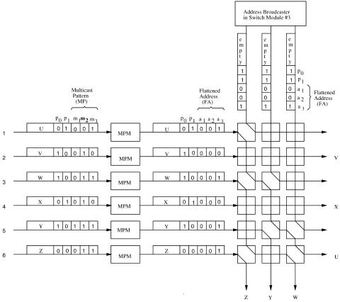
Figure 6.17 shows an example of how cells are routed in a switch module. Cells U, V, W, X, Y, and Z arrive at inputs 1 to 6, respectively, and are to be routed in switch module 3. In the cell header, there is a 3-bit multicast

Fig. 6.16 Switching condition of the switch element ŽSWE..

pattern Žm3 m2 m1 . and a 2-bit priority field Ž p1 p0 .. If a cell is to be sent to an output of this switch module, its m3 bit will be set to 1. Among these six cells, cells U, V, and X are for unicast, where only one bit in the multicast pattern is set to 1. The other three cells are for multicast, where more than one bit in the multicast pattern is set to 1. It is assumed that a smaller priority value has a higher priority level. For instance, cell Z has the highest priority level Ž00. and empty cells transmitted from the address broadcaster have the lowest priority level Ž11.. The MPM performs a logic AND function for each cell’s multicast pattern with a fixed pattern of 100. For instance, after cell W passes through the MPM, its multicast pattern Ž110. becomes 100 Ža3 a2 a1 ., which has only one bit set to 1 and is taken as the flattened address. When cells are routed in the SWE array, their routing paths are determined by the state of SWEs, which are controlled according to the rules in Figure 6.16. Since cells V and X are not destined for this group, the SWEs they pass remain in a cross state. Consequently, they are routed to the right side of the module and are discarded. Since there are only three routing links in this example, while there are four cells destined to this switch module, the one with the lowest priority Ži.e., cell U . loses contention to the other three and is discarded.

Since the crossbar structure inherits the characteristics of identical and short interconnection wires between switch elements, the timing alignment for the signals at each SWE is much easier than that of other types of

160 KNOCKOUT-BASED SWITCHES

Fig. 6.17 An example of routing a multicast cell.

interconnection network, such as the binary network, the Clos network, and so on. The unequal length of the interconnection wires increases the difficulty of synchronizing the signals, and, consequently limits the switch fabric’s size, as with the Batcher banyan switch. The SWEs in the switch modules only communicate locally with their neighbors, as do the chips that contain a two-dimensional SWE array. The switch chips do not need to drive long wires to other chips on the same printed circuit board. Note that synchronization of data signals at each SWE is only required in each individual switch module, not in the entire switch fabric.

6.3.3 Translation Tables

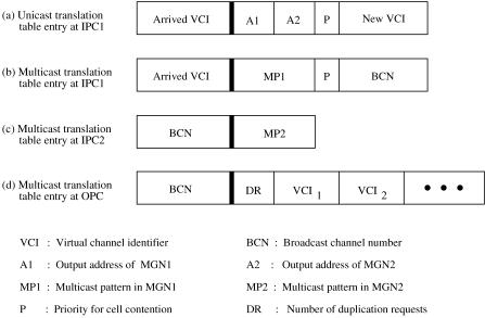
The tables in the IPC, MTT, and the OPC ŽFig. 6.18. contain information necessary to properly route cells in the switch modules of MGN1 and MGN2, and to translate old VCI values into new VCI values. As mentioned above, cell routing in the MGNs depends on the multicast pattern and priority

Fig. 6.18 Translation tables in the IPC, MTT, and OPC.

values that are attached in front of the incoming cell. To reduce the translation table’s complexity, the table contents and the information attached to the front of cells are different for the unicast and multicast calls.

In a point-to-point ATM switch, an incoming cell’s VCI on an input line can be identical with other cells’ VCIs on other input lines. Since the VCI translation table is associated with the IPC on each input line, the same VCI values can be repeatedly used for different virtual circuits on different input lines without causing any ambiguity. But cells that are from different virtual circuits and destined for the same output port need different translated VCIs.

In a multicast switch, since a cell is replicated into multiple copies that are likely to be transmitted on the same routing link inside a switch fabric, the switch must use another identifier, the broadcast channel number ŽBCN., to uniquely identify each multicast connection. In other words, the BCNs of multicast connections have to be different from each other, which is unlike the unicast case, where a VCI value can be repeatedly used for different connections at different input lines. The BCN can either be assigned during call setup or be defined as a combination of the input port number and the VPIrVCI value.

For the unicast situation, upon a cell’s arrival, its VCI value is used as an index to access the necessary information in the IPC’s translation table, such as the output addresses in MGN1 and MGN2, a contention priority value, and a new VCI, as shown in Figure 6.19Ža.. The output address of MGN1,

162 KNOCKOUT-BASED SWITCHES

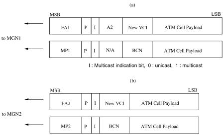
Fig. 6.19 Unicast and multicast cell formats in Ža. MGN1, Žb. MGN2.

A1, is first decoded into a flattened address, which has K bits and is put into the MP1 field in the cell header, as shown in Figure 6.19Ža.. The MP1 and P are used for routing cells in the MGN1, and A2 is used for routing cells in the MGN2. The I bit is the multicast indication bit, which is set to 0 for unicast and 1 for multicast. When a unicast cell arrives at the MTT, the A2 field is simply decoded into a flattened address and put into the MP2 field as the routing information in MGN2. Thus, no translation table in the MTT is needed for unicast cells. Note that A2 is not decoded into a flattened address until it arrives at the MTT. This saves some bits in the cell header Že.g., 27 bits for the above example of a 1024 1024 switch. and thus reduces the required operation speed in the switch fabric. The unicast cell routing format in MGN2 is shown in Figure 6.19Žb..

For the multicast situation, besides the routing information of MP1, MP2, and P, the BCN is used to identify cells that are routed to the same output group of a switch module. Similarly to the unicast case, an incoming cell’s VCI is first used to look up the information in the translation table in the IPC, as shown in Figure 6.18Žb.. After a cell has been routed through MGN1, MP1 is no longer used. Instead, the BCN is used to look up the next routing information, MP2, in the MTT, as shown in Figure 6.18Žc.. The cell formats for a multicast call in MGN1 and MGN2 are shown in Figure 6.19Ža. and Žb.. The BCN is further used at the OPC to obtain a new VCI for each duplicated copy that is generated by a cell duplicator at the OPC. The entry for the multicast translation table in the OPC is shown in Figure 6.18Žd..

Note that the in MTTs that are connected to the same MGN2 contain identical information, because the copy of a multicast cell can appear randomly at any one of L1 M output links to MGN2. As compared to those in w18, 26x, the translation table size in the MTT is much smaller. This is because the copy of a multicast cell can only appear at one of L1 M output links in the MOBAS, vs. N links in w18, 26x, resulting in fewer table entries in the MTT. In addition, since the VCI values of replicated copies are not stored in the MTT’s, the content of each table entry in the MTT is also less.

6.3.4 Multicast Knockout Principle

A new multicast knockout principle, an extension of generalized knockout principle, has been applied to the two-stage MOBAS to provide multicasting capability. Since the switch module ŽSM. in the MGN performs a concentration function Že.g., N to L1 M ., it is also called a concentrator.

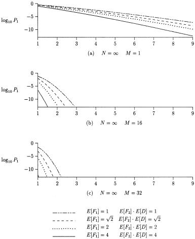
6.3.4.1 Cell Loss Rate in MGN1 In the analysis, it is assumed that the traffic at each input port of the MOBAS is independent of that at the other inputs, and replicated cells are uniformly delivered to all output groups. The average cell arrival rate, , is the probability that a cell arrives at an input port in a given cell time slot. It is assumed that the average cell replication in MGN1 is Ew F1 x, the average cell replication in MGN2 is Ew F2 x, the average cell duplication in the OPC is Ew Dx, and the random variables F1, F2 , and D are independent of each other.

Every incoming cell is broadcast to all concentrators ŽSMs., and is properly filtered at each concentrator according to the multicast pattern in the cell header. The average cell arrival rate, p, at each input of a concentrator is

p s Ew F1 x , K

where K Žs NrM . is the number of concentrators in MGN1. The probability Ž Ak . that k cells are destined for a specific concentrator of MGN1 in a given time slot is

Ak s žNk / pk Ž1 y p. Nyk

s žNk /ž Ew FN1 x M /k ž1 y Ew FN1 x M /Nyk , 0 F k F N, Ž6.8.

where Ew F1 x MrN is the probability of a cell arriving at the input of a specific concentrator in MGN1.

164 KNOCKOUT-BASED SWITCHES

As N ™ , Ž6.8. becomes

where should satisfy the following condition for a stable system:

Ew F1 x Ew F2 x Ew Dx 1.

Since there are only L1 M routing links available for each output group, if more than L1 M cells are destined for this output group in a cell time slot, excess cells will be discarded and lost. The cell loss rate in MGN1, P1, is

Ew F2 xEw Dx to allow for the cell replication in MGN2 and the OPC. In other words, a cell lost in MGN1 could be a cell that would have been replicated in MGN2 and the OPC. The denominator in Ž6.10., NpEw F2 xEw Dx, is the average number of cells effectively arriving at a specific concentrator

Note that Ž6.12. is similar to the equation for the generalized knockout principle, except that the parameters in the two equations are slightly different due to the cell replication in MGN1 and MGN2 and to the cell duplication in the OPC.

Figure 6.20 shows the plots of the cell loss probability at MGN1 vs. L1 for various fanout values and an offered load Žs Ew F1 xEw F2 xEw Dx. of 0.9 at each output port. Again it shows that as M increases Ži.e., more outputs are sharing their routing links., the required L1 value decreases for a given cell loss rate. The requirements on the switch design parameters M and L1 are more stringent in the unicast case than in the multicast. Since the load on MGN1 decreases as the product of the average fanouts in MGN2 and the

Fig. 6.20 Cell loss probability vs. the group expansion ratio L1in MGN1.

166 KNOCKOUT-BASED SWITCHES

OPC increases, the cell loss rate of MGN1 in the multicast case is lower than that in the unicast case. The replicated cells from a multicast call will never contend with each other for the same output group Žconcentrator., since the MOBAS replicates at most one cell for each output group. In other words, an MGN1 that is designed to meet the performance requirement for unicast calls will also meet the one for calls.

6.3.4.2 Cell Loss Rate in MGN2 Special attention is required when analyzing the cell loss rate in MGN2, because the cell arrival pattern at the inputs of MGN2 is determined by the number of cells passing through the corresponding concentrator in MGN1. If there are l Žl F L1 M . cells arriving at MGN2, these cells will appear at the upper l consecutive inputs of MGN2. If more than L1 M cells are destined for MGN2, only L1 M cells will arrive at MGN2’s inputs Žone cellper input port., while excessive cells are discarded in MGN1.

The cell loss rate of a concentrator in MGN2 is assumed to be P2 , and the probability that l cells arrive at a specific concentrator in MGN2 to be Bl. Both P2 and Bl depend on the average number of cells arriving at the inputs of MGN2 Ži.e., the number of cells passing through the corresponding concentrator in MGN1.. This implies that P2 is a function of Ak in Ž6.8.. In order to calculate P2 , the probability of j cells arriving at MGN2, denoted as Ij, is found to be

consecutive inputs of MGN2. Since how and where the cells appear at the MGN2’s inputs does not affect the cell loss performance, the analysis can be simplified by assuming that a cell can appear at any input of the MGN2.

Let us denote by Bl j the probability that l cells arrive at the inputs of a specific concentrator in MGN2 for given j cells arrived at MGN2. Then,

Bl j s žlj /ql Ž1 y q. jyl , 0 F j F L1 M, 0 F l F j,

where q is equal to Ew F2 xrM under the assumption that replicated cells are uniformly delivered to the M concentrators in MGN2.

If no more than L2 cells arrive at MGN2 Ž0 F j F L2 ., no cell will be discarded in MGN2, because each concentrator can accept up to L2 cells during one cell time slot. If more than L2 cells arrive at MGN2 Ž L2 F j F L1 M ., cell loss will occur in each concentrator with a certain probability.