Broadband Packet Switching Technologies

66 INPUT-BUFFERED SWITCHES

The scheduling of a given time slot in RRGS consists of N phases. In each phase, one input chooses one of the remaining outputs for transmission during that time slot. A phase consists of the request from the input module ŽIM. to the RR arbiter, RR selection, and acknowledgement from the RR arbiter to the IM. The RR order in which inputs choose outputs shifts cyclically for each time slot, so that it ensures equal access for all inputs.

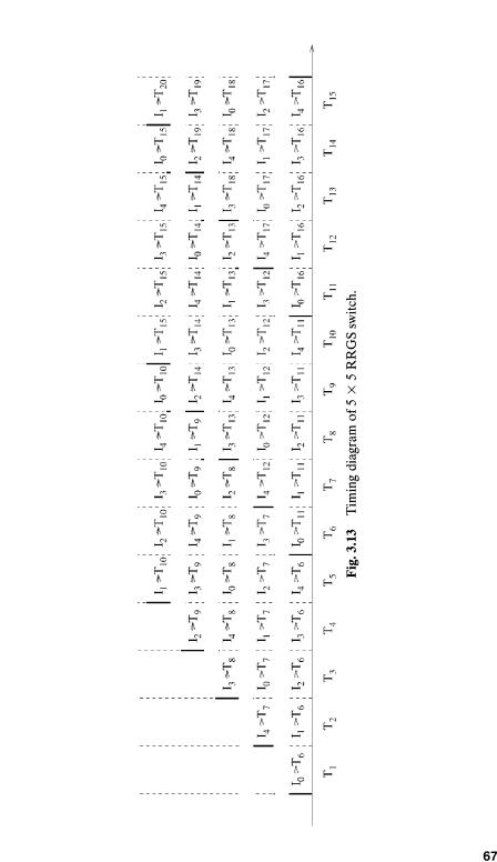
Now, we describe pipelined RRGS by applying the nonpipelined concept. We assume that N is an odd number to simplify the discussion. When N is an even number, the basic concept is the same, but there are minor changes. N separate schedules are in progress simultaneously, for N distinct time slots in the future. Each phase of a particular schedule involves just one input. In any given time slot, other inputs may simultaneously perform the phases of schedules for other distinct time slots in the future. While N time slots are required to complete the N phases of a given schedule, N phases of N different schedules may be completed within one time slot using a pipeline approach, and computing the N schedules in parallel. But this is effectively equivalent to the completion of one schedule every time slot. In RRGS, a specific time slot in the future is made available to the inputs for scheduling in a round-robin fashion. Input i, which starts a schedule for the kth time slot Žin the future., chooses an output in a RR fashion, and sends to the next input, Ži q 1. mod N, a set Ok that indicates the remaining output ports that are still free to receive packets during the kth time slot. Any input i, on receiving from the previous input, Ži y 1. mod N, the set Ok of available outputs for the kth time slot, chooses one output if possible from this set, and sends to the next input, Ži q 1. mod N, the modified set Ok , if input i did not complete the schedule for the kth time slot, Tk . An input i that completes a schedule for the kth time slot should not forward the modified set Ok to the next input, Ži q 1. mod N. Thus input Ži q 1. mod N, which did not receive the set Ok in the current time slot, will be starting a new schedule Žfor a new time slot. in the next time slot. Step 1 of RRGS implies that an input refrains from forwarding Ok once in N time slots. The input i that does not forward Ok should be the last one that chooses an output for the kth time slot. Thus, since each RR arbiter has only to select one candidate within one time slot, RRGS dramatically relaxes the scheduling time constraint compared with iSLIP and DRRM.

Figure 3.13 shows an example of a timing diagram of a pipelined 5 5 RRGS algorithm.

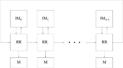
A simple structure for the central controller that executes the RRGS algorithm is shown in Figure 3.14. A RR arbiter associated to each input module communicates only with the RR arbiters associated to adjacent input modules, and the complex interconnection between input and output modules is avoided. It stores addresses of the reserved outputs into the memory ŽM..

68 INPUT-BUFFERED SWITCHES

The price that RRGS pays for its simplicity is the additional pipeline delay, which is on average equal to Nr2 time slots. This pipeline delay is not critical for the assumed very short packet transmission time. Smiljanic´ et al. w30x showed that RRGS provides better performance than iSLIP with one iteration for a heavy load.

Smiljanic´ also proposed so-called weighted RRGS ŽWRRGS., which guarantees prereserved bandwidth w31x, while preserving the advantage of RRGS. WRRGS can flexibly share the bandwidth of any output among the inputs.

3.3.6 Design of Round-Robin Arbiters r Selectors

A challenge to building a large-scale switch lies in the stringent arbitration time constraint for output contention resolution. This section describes how to design the RR-based arbiters.

3.3.6.1 Bidirectional Arbiter A bidirectional arbiter for output resolution control operates using three output-control signals, DL, DH, and UH as shown in Figure 3.15 w10x. Each signal is transmitted on one bus line. DL and DH are downstream signals, while UH is the upstream signal.

The three signal bus functions are summarized as follows:

DL: Selects highest requested crosspoint in group L.

DH: Selects highest requested crosspoint in group H.

UH: Identifies whether group H has request or not.

Fig. 3.15 Block diagram of the bidirectional arbiter. Ž 1994 IEEE..

70 INPUT-BUFFERED SWITCHES

TABLE 3.2 A Part of the Logic Table of the Bidirectional Arbiter

aGroup Indication indicating which group the crosspoint belongs to.

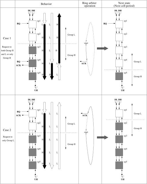
The arbitration procedure can be analyzed into two cases in Figure 3.15. Case 1 has group H active or both L and H active. In this case, the highest request in group H will be selected. Case 2 has only group L active. In that case, the highest request in group L will be selected.

In case 1, the DH signal locates the highest crosspoint in Group H, xp4, and triggers the ACK signal. The UH signal indicates that there is at least one request in group H to group L. The DL signal finds the highest crosspoint, xp1, in group L, but no ACK signal is sent from xp1, because of the state of the UH signal. In the next cell period, xp1 to xp4 form group L, and xp5 is group H.

In case 2, the UH signal shows that there is no request in group H; the DL signal finds the highest request in group L, xp1, and triggers the ACK signal.

Note that both selected crosspoints in case 1 and case 2 are the same crosspoints that would be selected by a theoretical RR arbiter.

The bidirectional arbiter operates two times faster than a normal ring arbiter Žunidirectional arbiter., but twice as many transmitted signals are required. The bidirectional arbiter can be implemented with simple hardware. Only 200 or so gates are required to achieve the distributed arbitration at each crosspoint, according to the logic table shown in Table 3.2.

3.3.6.2 Token Tunneling This section introduces a more efficient arbitration mechanism called token tunneling w4x. Input requests are arranged into groups. A token starts at the RR pointer position and runs through all

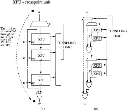
Fig. 3.16 The token tunneling scheme. Ž 2000 IEEE..

requests before selecting the one with the highest priority. As shown in Figure 3.16Ža., when the token arrives in a group where all requests are 0, it can skip this group taking the tunnel directly from the input of the group to the output. The arbitration time thus becomes proportional to the number of groups, instead of the number of ports.

Suppose each group handles n requests. Each crosspoint unit ŽXPU. contributes a two-gate delay for arbitration. The token rippling through all the XPUs in the group where the token is generated and all the XPUs in the group where the token is terminated contributes a 4 n-gate delay. There are altogether Nrn groups, and at most Nrn y 2 groups will be tunneled through. This contributes a 2Ž Nrn y 2.-gate delay. Therefore, the worst case

group. This occurs when there is only one active request and it is at the farthest position from the round-robin pointer or example, the request is at the bottommost XPU while the round-robin pointer points to the topmost one.

By tunneling through smaller XPU groups of size g and having a hierarchy of these groups as shown in Figure 3.16Žb., it is possible to further reduce the

d s log 2Žnrg. . The hierarchical method basically decreases the time spent in the group where the token is generated and in the group where the token is terminated. For N s 256, n s 16, and g s 2, the basic token tunneling method requires a 92-gate delay, whereas the hierarchical method requires only a 51-gate delay.

3.4 OUTPUT-QUEUING EMULATION

The major drawback of input queuing is that the queuing delay between inputs and outputs is variable, which makes delay control more difficult. Can an input output-buffered switch with a certain speedup behave identically 4 to an output-queued switch? The answer is yes, with the help of a better scheduling scheme. This section first introduces some basic concepts and then highlights some scheduling schemes that achieve the goal.

3.4.1 Most-Urgent-Cell-First Algorithm (MUCFA)

The MUCFA scheme w29x schedules cells according to their urgency. A shadow switch with output queuing is considered in the definition of the urgency of a cell. The urgency, which is also called the time to leave ŽTL., is the time after the present that the cell will depart from the output-queued ŽOQ. switch. This value is calculated when a cell arrives. Since the buffers of the OQ switch are FIFO, the urgency of a cell at any time equals the number of cells ahead of it in the output buffer at that time. It gets decremented after every time slot. Each output has a record of the urgency value of every cell destined for it. The algorithm is run as follows:

1.At the beginning of each phase, each output sends a request for the most urgent cell Ži.e., the one with the smallest TL. to the corresponding input.

2.If an input receives more than one request, then it will grant to that output whose cell has the smallest urgency number. If there is a tie between two or more outputs, a supporting scheme is used. For example, the output with the smallest port number wins, or the winner is selected in a RR fashion.

3.Outputs that lose contention will send a request for their next most urgent cell.

4.The above steps run iteratively until no more matching is possible. Then cells are transferred, and MUCFA goes to the next phase.

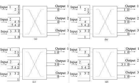
An example is shown in Figure 3.17. Each number represents a queued cell, and the number itself indicates the urgency of the cell. Each input maintains three VOQs, one for each output. Part Ža. shows the initial state of

4 Under identical inputs, the departure time of every cell from both switches is identical.

Fig. 3.17 An example of two phases of MUCFA.

the first matching phase. Output 1 sends a request to input 1, since the HOL cell in VOQ1, 1 is the most urgent for it. Output 2 sends a request to input 1, since the HOL cell in VOQ1, 2 is the most urgent for it. Output 3 sends a request to input 3, since the HOL cell in VOQ3, 3 is the most urgent for it. Part Žb. illustrates matching results of the first phase, where cells from VOQ1, 1, VOQ2, 2 , and VOQ3, 3 are transferred. Part Žc. shows the initial state of the second phase, while part Žd. gives the matching results of the second phase, in which HOL cells from VOQ1, 2 and VOQ3, 3 are matched.

It has been shown that, under an internal speedup of 4, a switch with VOQ and MUCFA scheduling can behave identically to an OQ switch, regardless of the nature of the arrival traffic.

3.4.2 Chuang et al.’s Results

This category of algorithms is based on an implementation of priority lists for each arbiter to select a matching pair w7x. The input priority list is formed by positioning each arriving cell at a particular place in the input queue. The relative ordering among other queued cells remains unchanged. This kind of queue is called a push-in queue. Some metrics are used for each arriving cell to determine the location. Furthermore, if cells are removed from the queue in an arbitrary order, we call it a push-in arbitrary out ŽPIAO. queue. If the cell at the head of queue is always removed next, we call it a push-in first out ŽPIFO. queue.

74 INPUT-BUFFERED SWITCHES

The algorithms described in this section also assume a shadow OQ switch, based on which the following terms are defined:

1.The time to lea®e TLŽc. is the time slot in which cell c would leave the shadow OQ switch. Of course, TLŽc. is also the time slot in which cell c must leave the real switch for the identical behavior to be achieved.

2.The output cushion OCŽc. is the number of cells waiting in the output

buffer at cell c’s output port that have a lower TL value than cell c. If a cell has a small Žor zero. output cushion, then it is urgent for it to be delivered to its output so that it can depart when its time to leave is reached. If it has a large output cushion, it may be temporarily set aside while more urgent cells are delivered to their outputs. Since the switch is work-conserving, a cell’s output cushion is decremented after every time slot. A cell’s output cushion increases only when a newly arriving cell is destined for the same output and has a more urgent TL.

3.The input thread ITŽc. is the number of cells ahead of cell c in its input priority list. ITŽc. represents the number of cells currently at the input that have to be transferred to their outputs more urgently than cell c. A cell’s input thread is decremented only when a cell ahead of it is transferred from the input, and is possibly incremented when a new cell arrives. It would be undesirable for a cell to simultaneously have a large input thread and a small output cushion the cells ahead of it at the input might prevent it from reaching its output before its TL. This motivates the definition of slackness.

4.The slackness LŽc. equals the output cushion of cell c minus its input thread, that is, LŽc. s OCŽc. y ITŽc.. Slackness is a measure of how large a cell’s output cushion is with respect to its input thread. If a cell’s slackness is small, then it is urgent for it to be transferred to its output. If a cell has a large slackness, then it may be kept at the input for a while.

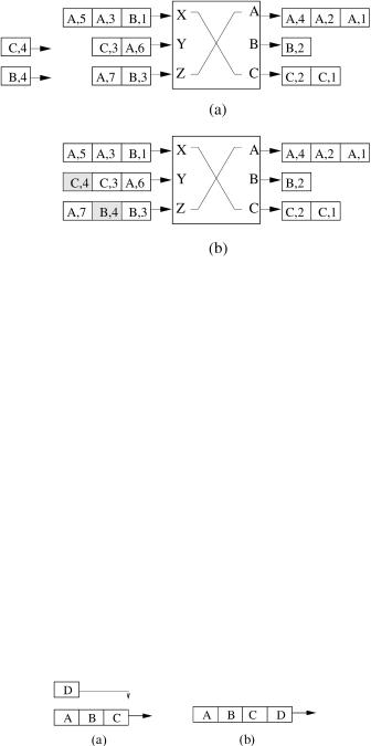
3.4.2.1 Critical Cell First (CCF) CCF is a scheme of inserting cells in input queues that are PIFO queues. An arriving cell is inserted as far from the head of its input queue as possible so that the input thread of the cell is not larger than its output cushion Ži.e., the slackness is positive.. Suppose that cell c arrives at input port P. Let x be the number of cells waiting in the output buffer at cell c’s output port. Those cells have a lower TL value than cell c or the output cushion OCŽc. of c. Insert cell c into Ž x q 1.th position from the front of the input queue at P. As shown in Figure 3.18, each cell is represented by its destined output port and the TL. For example, cell Ž B, 4. is destined for output B and has a TL value equal to 4. Part Ža. shows the initial state of the input queues. Part Žb. shows the insertion of two incoming cells ŽC, 4. and Ž B, 4. to ports Y and Z, respectively. Cell ŽC, 4. is inserted at

Fig. 3.18 Example of CCF priority placement.

the third place of port Y, and cell Ž B, 4. at the second place of port Z. Hence, upon arrival, both cells have zero slackness. If the size of the priority list is less than x cells, then place c at the end of the input priority list. In this case, cell c has a positive slackness. Therefore, every cell has a nonnegative slackness on arrival.

3.4.2.2 Last In, Highest Priority (LIHP) LIHP is also a scheme of inserting cells at input queues. It was proposed mainly to show and demonstrate the sufficient speedup to make an input output queued switch emulate an output-queued switch. LIHP places a newly arriving cell right at the front of the input priority list, providing a zero input thread wITŽc. s 0x for the arriving cell. See Figure 3.19 for an example. The scheduling in every arbitration phase is a stable matching based on the TL value and the position

Fig. 3.19 An example of placement for LIHP. Ža. The initial state. Žb. The new cell is placed at the highest-priority position.