Broadband Packet Switching Technologies

Fig. 6.28 Fault location test for a cross-stuck SWE by moving the square block around in the SWE array.

Figure 6.28 shows an example of the fault location test for a CS SWE ŽCS test.. This test can also be used to locate a HS SWE. To diagnose the SWEs in the three uppermost rows, the priorities of the test cells, X3, X2, X1, V1, V2, and V3, are arranged in descending order. These cells’ FAs are set to be identical, but the FAs of test cells X4, X5, and X6 are set to be different. The CS test forces all SWEs in the square block Ž3 3 in this example. to a toggle state and all other SWEs to a cross state. If there exists a CS in this square block, the output pattern will be different from the expected one. For offline testing of a switch module, at least NrL1 M tests are required in MGN1, and L1 MrL2 tests in MGN2.

6.4.3.2 Vertical-Stuck and Horizontal-Stuck Cases If a VS or an HS fault exists in the SWE array, cells that pass through the faulty SWE will be corrupted as shown in Figure 6.24 and Figure 6.25. Once a VS fault is

178 KNOCKOUT-BASED SWITCHES

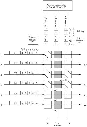
Fig. 6.29 Reconfiguration by isolating a faulty column caused by a vertical s stuck SWEŽ4, 2..

detected by the FD at MTTs or OPCs, the information about the faulty column is known immediately. This information is sufficient to reconfigure the switch network. For example, if the jth column contains a VS Ž j s 2 in Figure 6.24., all the SWEs in the jth column are forced to a cross state, so that the jth column is isolated. For instance, Figure 6.29 shows the reconfiguration with the second column isolated. Of course, the cell loss performance is degraded because of the reduction of available routing links.

Special attention is needed for a HS fault, because we must locate exactly the faulty SWE prior to proper reconfiguration. Once a HS fault is detected, we have the information about the faulty row automatically. What we need is the column information. In order to locate the fault, we define a fault location test ŽHS test. for it.

The HS test sets the test cells’ FA, priority, and source address to appropriate values such that all SWEs on the faulty row are forced to a

toggle state. Let us consider an HS test for the ith row of the SWE array. The FA of test cells from all MPMs except the ith MPM are set to all zeros Žfor mismatching purposes., while the test cell’s FA from the ith MPM is set to be identical to that of the test cells from the AB. All test cells’ source addresses are set to their row numbers or column numbers, depending on whether they are fed to the SWE array horizontally or vertically. Priorities of the test cell from the ith MPM and broadcast test cells from AB are set in descending order. Normally, the priority of the test cell from the ith MPM is the highest,the broadcast test cell from the first column is the second highest, the broadcast test cell from the second column is the third highest, and so on.

Fig. 6.30 Fault location test for a horizontal-stuck SWE by forcing the SWEs in the faulty row to a toggle state.

180 KNOCKOUT-BASED SWITCHES

With this arrangement, the cell from the ith MPM will appear at the first output link, while the broadcast cell from the r th AB will appear at the Žr q 1.th output link or the ith discarding output. The FDs at the output links examine the source address SA field to locate the faulty column that contains the HS SWE. If the jth column contains a HS SWE, the test cell from the ith MPM will appear at the first output link, and the test cell Vr broadcast from the r th AB Ž1 F r F j y 1. will appear at the Žr q 1.th output link. The test cell Vj broadcast from the jth AB will be corrupted and appear at the ith discarding output. The test cell, Vjqs broadcast from the Ž j q s.th AB Ž1 F s F L1 M y j. will appear at the Ž j q s.th output link. If a HS SWE is on the last column, the test cell from the r th AB will appear at the Žr q 1.th output link, and the test cell broadcast from the rightmost AB appears at the ith discarding output and is corrupted.

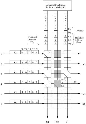
Figure 6.30 shows a test example where a HS SWE exists in the fourth row and all SWEs in the fourth row are forced to a toggle state to locate the HS

Fig. 6.31 Reconfiguration by isolating the upper column of the horizontal-stuck SWEŽ4, 2..

SWE. For example, if SWEŽ4, 2. is HS, cell V3 Žinstead of cell V2. will appear at output link 3; cell V2, which is corrupted, will appear at the 4th discarding output.

After locating the HS fault, say at SWEŽi, j., we can reconfigure the SWE array by forcing SWEŽi, j. to a toggle state and the switch elements that are in the same column and are above the faulty SWE wSWEŽk, j., 1 F k F i y 1x to a cross state, so that cells will not be affected by the HS SWEŽi, j.. Figure 6.31 shows an example of the reconfiguration for a HS at SWEŽ4, 2..

6.4.4 Performance Analysis of Reconfigured Switch Module

In this subsection, we show the graceful cell loss performance degradation of a SM under faulty conditions. The cell loss rate of each input under different faults is calculated. For simplicity, it is assumed that the SM has an N L SWE array, that all incoming cells have the same priority and have a higher priority than broadcast cells from the AB, and that the traffic at each input port of the MOBAS is independent of that at the other inputs. The average cell arrival rate, , is the probability that a cell arrives at an input port in a given time slot. It is also assumed that cells are uniformly delivered to all output ports and that there is only point-to-point communication, which gives the worst-case performance analysis. As a result, the traffic at each input of the SM has an identical Bernoulli distribution with rN as its average cell arrival rate.

PLŽk. is defined as the cell loss rate of the kth input with an expansion ratio L under a fault-free condition. The cell loss rates of the uppermost L inputs are zero, meaning that cells from these inputs are always delivered successfully, or

PLŽ k . s 0, 1 F k F L.

The cell loss rates of the remaining inputs, from input L q 1 to input N, are

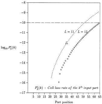
Fig. 6.32 Cell loss rate of each input port after cross-reconfiguration. Ž 1994 IEEE..

The probability PŽ A. is considered as the cell loss rate improvement of the kth input

Figure 6.32 shows the cell loss rate of each input after the SWE array is reconfigured. Here, the MOBAS is assumed to be a single stage with a size of 64 64 and an expansion ratio L of 12. The faulty SWE is assumed to be SWEŽ35, 12.. For those inputs above the faulty input Ž35., the cell loss rates are the same as in the fault-free case, while the faulty input’s cell loss rate is equal to that of the L s 11 fault-free case. The inputs below the faulty one Žfrom 36 to 64. have almost the same cell loss rates as in the fault-free case, since the improvement PŽ A. is very small.

6.4.4.2 Vertical-Stuck Case When there is a VS SWE in the jth column, all the SWEs in that column are forced to a cross state to isolate the jth column, as shown in Figure 6.29 Ž j s 2.. This column isolation prevents cells from being corrupted, but reduces available routing links from L to L y 1. Therefore, after the reconfiguration, the cell loss rate of each input is slightly increased to the following:

PLŽ k . s PLy1 Ž k . , 1 F k F N.

Note that the effect on the cell loss performance degradation is independent of the faulty link’s position. The cell loss rates after the reconfiguration are

184 KNOCKOUT-BASED SWITCHES

equal to those of the fault-free L s 11 case, regardless of the row position of the faulty link.

6.4.4.3 Horizontal-Stuck SWE Case Figure 6.31 shows a reconfiguration example of HS SWEŽ4, 2.. Let us consider an HSŽi, j. case: the cell loss rates of all inputs above the ith one are equal to those of the fault-free Ž L y 1. case, while the ith input has no cell loss. And the cell loss rates of all inputs below the ith one are almost equal to those of the fault-free Ž L y 1. case. Incoming cells from all inputs above the ith one can only be routed to L y 1 output links, and the ith input always occupies one of j output links Žfrom the first to the jth..

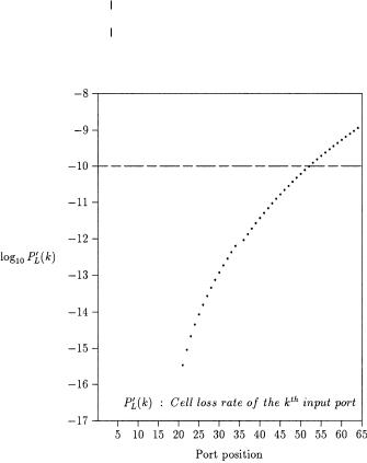
Fig. 6.33 Cell loss rate of each input port after partial column isolation.

Figure 6.33 shows the cell loss rates of inputs of the switch module with a HS SWE. The cell loss rates of all inputs above the faulty one Ži s 35. are equal to those of fault-free L s 11 case, while the faulty input has no cell loss. The cell loss rates of the inputs below the faulty one are almost equal to those of the fault-free L s 11 case, because one of j output links is always occupied by the cells from the faulty input, and they are independent of the faulty input’s cell arrival pattern.

From the above analysis it can be concluded that under the single-fault condition, the worst cell loss performance degradation corresponds to the loss of one output link. Note that these cell loss rates are not the average rate of the entire MOBAS but that of the SM with a faulty SWE. When an input experiences cell loss performance degradation due to a faulty SWE, it corresponds to one output link loss in the worst case. Thus, if we add one more column of SWEs for each switch module, which corresponds to less than 2% hardware overhead in MGN1 and less than 9% hardware overhead in MGN2, under any kind of single-fault condition, the MOBAS can still have as good cell loss performance as the originally designed, fault-free system.

6.5 APPENDIX

Let us consider an ATM switch as shown in Figure 6.10, and assume that cells arrive independently from different input ports and are uniformly delivered to all output ports. The variables used are defined as follows.

N: the number of a switch’s input ports or output ports

M: the number of output ports that are in the same group

L: the group expansion ratio

: the offered load of each input port, or the average number of cells that arrive at the input port in each cell time slot

rN: the average number of cells from each input port destined for an output port in each cell time slot

MrN: the number of cells from each input port destined for an output group in each cell time slot

Pk : the probability that k cells arrive at an output group in each cell time slot

: the average number of cells from all input ports that are destined for an output group in each cell time slot

: the average number for cells from all input ports that have arrived at an output group in each cell time slot

186 KNOCKOUT-BASED SWITCHES

Then Pk is given by the following binomial probability:

Pk s žNk /ž NM /k ž1 y NM /Nyk , k s 0, 1, . . . , N,

and we have

ksLMq1

Since at most LM cells are sent to each output group in each cell time slot, the excess cells will be discarded and lost. The cell loss probability is