Broadband Packet Switching Technologies

determines that the HOL cell has been successfully routed to RMs 1 and K but discarded in RM 3 and will retransmit in the next time slot.

7.3 IMPLEMENTATION OF INPUT PORT CONTROLLER

Figure 7.5 shows a block diagram of the IPC. For easy explanation, let us assume the switch has 256 input ports and 256 output ports, and every 16 successive output ports are in one group. A major difference between this IPC and traditional ones is the addition of the multicast contention resolution unit ŽMCRU., shown in a dashed box. It determines, by comparing K feedback priorities with the local priority of the HOL cell, whether or not the HOL cell has been successfully routed to all necessary output groups.

Let us start from the left, where the input line from the SONET ATM network is terminated. Cells 16 bits wide are written into an input buffer.

Fig. 7.5 Implementation of the input port controller with N s 256, M s 16. Ž 1997 IEEE..

198 THE ABACUS SWITCH

The HOL cell’s VPIrVCI is used to extract necessary information from a routing table. This information includes a new VPIrVCI for unicast connections; a BCN for multicast connections, which uniquely identifies each multicast call in the entire switch; a MP for routing cells in the MGN; and the connection priority C. This information is then combined with a priority field to form the routing information, as shown in Figure 7.3.

As the cell is transmitted to the MGN through a parallel-to-serial converter ŽPrS., the cell is also temporarily stored in a one-cell buffer. If the cell fails to route successfully through the RMs, it will be retransmitted in the next cell cycle. During retransmission, it is written back to the one-cell buffer in case it fails to route through again. The S down counter is initially loaded with the input address and decremented by one at each cell clock. The R down counter is initially set to all 1s and decreased by one every time the HOL cell fails to transmit successfully. When the R-counter reaches zero, it will remain at zero until the HOL cell has been cleared and a new cell becomes the HOL cell.

K feedback priority signals, FP1 to FPK , are converted to 16-bit-wide signals by the serial-to-parallel converters ŽSrP. and latched at the 16-bit registers. They are simultaneously compared with the HOL cell’s local priority ŽLP. by K comparators. Recall that the larger the priority value is, the lower the priority level is. If the value of FPj is larger than or equal to LP, the jth comparator’s output is asserted low, which will then reset the MPj bit to zero regardless of what its value was Ž0 or 1.. After the resetting operation, if any one of the MPj bits is still 1, indicating that at least one HOL cell did not get through the RM in the current cycle, the resend signal will be asserted high and the HOL cell will be retransmitted in the next cell cycle with the modified multicast pattern.

As shown in Figure 7.5, there are K sets of SrP, FP register, and comparator. As a switch size increases, the number of output groups, K, also increases. However, if the time permits, only one set of this hardware is required for time-division multiplexing the operation of comparing the local priority value, LP, with K feedback priority values.

7.4 PERFORMANCE

This section discusses the performance analysis of the abacus switch. Both simulation and analytical results are given for comparison. Simulation results are obtained with a 95% confidence interval, with errors not greater than 10% for the cell loss probability or 5% for the maximum throughput and average cell delay.

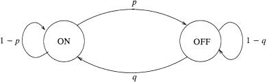
Figure 7.6 considers an on off source model in which an arrival process to an input port alternates between on Žactive. and off Židle. periods. A traffic source continues sending cells in every time slot during the on period, but stops sending cells in the off period. The duration of the on period is

PERFORMANCE 199

Fig. 7.6 On off source model.

determined by a random variable X g 1, 2, . . . 4, which is assumed to be geometrically distributed with a mean of cells. Similarly, the duration of the off period is determined by a random variable Y g 0, 1, 2, . . . 4, which is also assumed to be geometrically distributed with a mean of cells. Define q as the probability of starting a new burst Žon period. in each time slot, and p as the probability of terminating a burst. Cells arriving at an input port are assumed to be destined for the same output. Thus, the probability that the on period lasts for a duration of i time slots is

Pr X s i4 s pŽ1 y p. iy1 , i G 1,

and we have

The probability that an off period lasts for j time slots is

7.4.1 Maximum Throughput

The maximum throughput of an ATM switch employing input queuing is defined by the maximum utilization at the output port. An input-buffered switch’s HOL blocking problem can be alleviated by speeding up the switch fabric’s operation rate or increasing the number of routing links with an expansion ratio L. Several other factors also affect the maximum throughput. For instance, the larger the switch size Ž N . or burstiness Ž ., the smaller the

200 THE ABACUS SWITCH

maximum throughput Ž max . will be. However, the larger the group expansion ratio Ž L. or group size Ž M . is, the larger the maximum throughput will be.

input output-buffered ATM switch for M s 1, an arbitrary group expansion ratio or speedup factor L, and an infinite N with random traffic. Pattavina w14x has obtained, through computer simulations, the maximum throughput of an input output-buffered ATM switch, using the channel grouping concept for an arbitrary group size M, L s 1, and an infinite N with random traffic. Liew and Lu w12x have obtained the maximum throughput of an asymmetric input-output-buffered switch module for arbitrary M and L, and N ™ with bursty traffic.

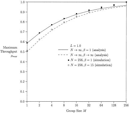
Figure 7.7 shows that the maximum throughput is monotonically increasing with the group size. For M s 1, the switch becomes an input-buffered switch, and its maximum throughput max is 0.586 for uniform random traffic

Fig. 7.7 Maximum throughput vs. group size, L s 1.0.

PERFORMANCE 201

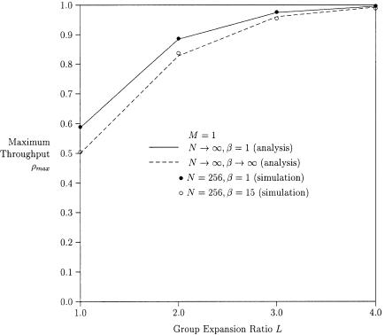
Fig. 7.8 Maximum throughput vs. group expansion ratio with M s 1.

Ž s 1., and 0.5 for completely bursty traffic Ž ™ .. For M s N, the switch becomes a completely shared-memory switch such as Hitachi’s switch w11x. Although it can achieve 100% throughput, it is impractical to implement a large-scale switch using such an architecture. Therefore, choosing M between 1 and N is a compromise between the throughput and the implementation complexity.

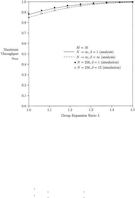
Figures 7.8 and 7.9 compare theoretical values and simulation values of the maximum throughput with different group expansion ratios L for M s 1 and M s 16, respectively. The theoretical values can be obtained from Liew and Lu’s analysis w12x.

A HOL virtual queue is defined as the queue that consists of cells at the HOL of input buffers destined for a tagged output group. For uniform random traffic, the average number of cells, EwC x, in the HOL virtual queue

PERFORMANCE 203

The maximum throughput of the proposed ATM switch can be obtained by considering the total number of backlogged cells in all K HOL virtual queues to be N. This means under a saturation condition, there is always a HOL cell at each input queue. Since it is assumed that cells are uniformly distributed over all output groups, we obtain

The maximum throughput can be obtained by equating Ž7.1. and Ž7.3. for

are more routing links available between input ports and output groups. However, since a larger L means higher hardware complexity, the value of L should be selected prudently so that both hardware complexity and the maximum throughput are acceptable. For instance, for a group size M of 16 Žfor input traffic with an average burst length of 15 cells., L has to be at least 1.25 to achieve a maximum throughput of 0.95. But for a group size M of 32 and the same input traffic characteristic, L need only be at least 1.125 to achieve the same throughput. Both analytical results and simulation results show that the effect of input traffic’s burstiness on the maximum throughput is very small. For example, the maximum throughput for uniform random traffic with M s 16 and L s 1.25 is 97.35%, and for completely bursty traffic is 96.03%, only a 1.32% difference. The discrepancy between theoretical and simulation results comes from the assumptions on the switch size N and . In the theoretical analysis, it is assumed that N ™ , ™ , but in the simulation it is assumed that N s 256, s 15. As these two numbers increase, the discrepancy decreases.

7.4.2 Average Delay

A cell may experience two kinds of delay while traversing the abacus switch: input-buffer delay and output-buffer delay. In the theoretical analysis, the buffer size is assumed to be infinite. But in the simulations, it is assumed that the maximum possible sizes for the input buffers and output buffers that can be sustained in computer simulations are Bi s 1024 and Bo s 256, respectively. Here, Bi is the input buffer size and Bo is the normalized output buffer size wi.e., the size of a physical buffer Ž4096. divided by M Ž16.x. Although finite buffers may cause cell loss, it is small enough to be neglected when evaluating average delay.

Let us assume each input buffer receives a cell per time slot with a probability , and transmits a cell with a probability . The probability is equal to 1.0 if there is no HOL blocking. But, as the probability of HOL blocking increases, will decrease. If , then the input buffer will

204 THE ABACUS SWITCH

rapidly saturate, and the delay at it will be infinite. The analytical results for uniform random traffic can be obtained from Chang et al.’s analysis w2x:

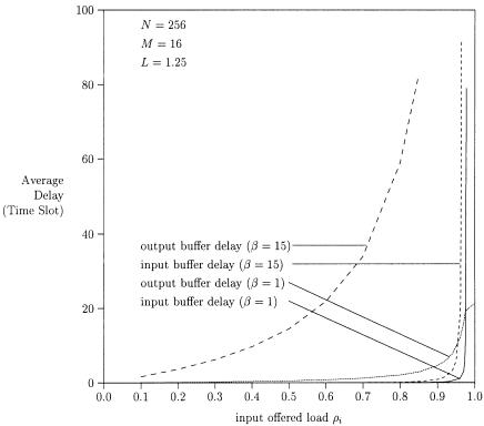
Note that the input buffer’s average delay is very small when the input offered load is less than the maximum saturation throughput. This results from the small HOL blocking probability before the saturated throughput. It also shows that the effect of the burstiness of input traffic on the input buffer’s average delay is very small when the traffic load is below the maximum throughput.

Figure 7.10 compares the average delay at the input and output buffers. Note that the input buffer’s average delay is much smaller than the output

Fig. 7.10 Comparison of average input buffer delay and average output buffer delay.

PERFORMANCE 205

buffer’s at traffic loads less than the saturated throughput. For example, for an input offered load i of 0.8 and an average burst length of 15, the output buffer’s average delay To is 58.8 cell times, but the input buffer’s average delay Ti is only 0.1 cell time.

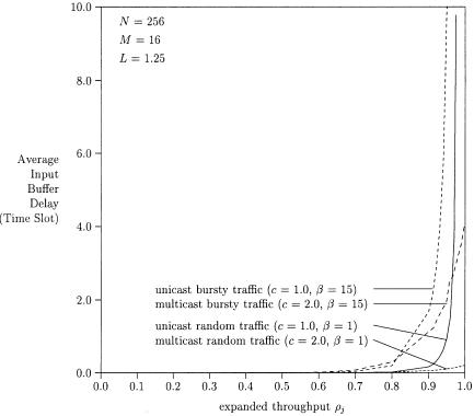
Figure 7.11 shows simulation results on the input buffer’s average delay vs. the expanded throughput j for both unicast and multicast traffic. It is assumed that the number of replicated cells is distributed geometrically with an average of c. The expanded throughput j is measured at the inputs of the SSM and normalized to each output port. Note that multicast traffic has a lower delay than unicast traffic, because a multicast cell can be sent to multiple destinations in a time slot, while a unicast cell can be sent to only one destination in a time slot. For example, assume that an input port i has 10 unicast cells and the other input port j has a multicast cell with a fanout of 10. Input port i will take at least 10 time slots to transmit the 10 unicast cells, while input port j can possibly transmit the multicast cell in one time slot.

Fig. 7.11 Average input buffer delay vs. expanded throughput for unicast and multicast traffic Žsimulation..

206 THE ABACUS SWITCH

7.4.3 Cell Loss Probability

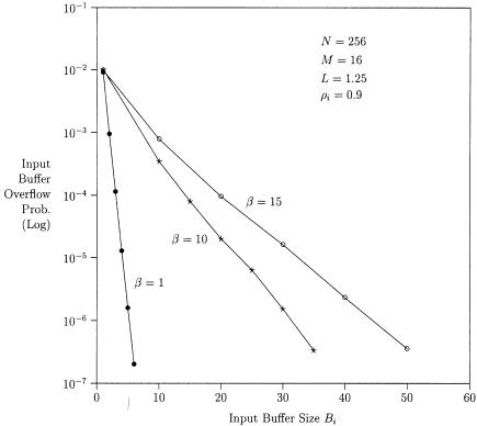
As suggested in w15x, there can be two buffer control schemes for an input output-buffered switch: the queue loss ŽQL. scheme and the backpressure ŽBP. scheme. In the QL scheme, cell loss can occur at both input and output buffers. In the BP scheme, by means of backward throttling, the number of cells actually switched to each output group is limited not only to the group expansion ratio Ž LM ., but also to the current storage capability in the corresponding output buffer. For example, if the free buffer space in the corresponding output buffer is less than LM, only the number of cells corresponding to the free space are transmitted, and all other HOL cells destined for that output group remain at their input buffers. The abacus switch can easily implement the backpressure scheme by forcing the AB in Figure 7.2 to send the dummy cells with the highest priority level, which will automatically block the input cells from using those routing links. Further-

Fig. 7.12 Input buffer overflow probability vs. input buffer size Žsimulation..