Broadband Packet Switching Technologies

buffers are used to store internally blocked cells so that the cell loss rate can be reduced. Scalability of the switch can be easily achieved by replicating the SEs. However, this type of switch suffers from low throughput and high transfer delay that is caused by the delay from multiple stages. To meet QoS requirements, some scheduling and buffer management schemes need to be installed at the internal SEs, which will increase the implementation cost.

2.2.3.2 Recirculation Buffered Switches This type of switch is proposed to overcome the output port contention problem. As shown in Figure 2.15Žb., the switch consists of both inputroutput ports and special ports called recirculation ports. When output port contention occurs, the switch allows the successful cell to go to the output port. Cells that have lost the contention are stored in a recirculation buffer and try again in the next time slot.

In order to preserve the cell sequence, a priority value is assigned to each cell. In each time slot, the priority level of the cells losing contention is increased by one so that these cells will have a better chance to be selected in the next time slot. If a cell has reached its highest priority level and the cell still has not gotten through, it will be discarded to avoid out-of-sequence errors.

The number of recirculation ports can be engineered to achieve acceptable cell loss rate. For instance, it has been shown that to achieve a cell loss rate of 10y6 at 80% load and Poisson arrivals, the ratio of recirculation ports to input ports must be 2.5. The Starlite switch w6x is an example of this type of switch.

The number of recirculation ports can be reduced dramatically by allowing more than one cell to arrive at the output port in each time slot. It has been shown that for a cell loss probability of 10y6 at 100% load and Poisson arrivals, the ratio of the recirculation ports to the input ports is reduced to 0.1 by allowing three cells arriving at each output port. The Sunshine w4x switch is an example of this switch type.

2.2.3.3 Crosspoint-Buffered Switches This type of switch, as shown in Figure 2.15Žc., is the same as the crossbar-based switch discussed in Section 2.2.2.

2.2.3.4 Input-Buffered Switches The input-buffered switch, as shown in Figure 2.15Žd., suffers from the HOL blocking problem and limits the throughput to 58.6% for uniform traffic. In order to increase the switch’s throughput, a technique called windowing can be employed, where multiple cells from each input buffer are examined and considered for transmission to the output port. But at most one cell will be chosen in each time slot. The number of examined cells determines the window size. It has been shown that by increasing the window size to two, the maximum throughput is increased to 70%. Increasing the window size does not improve the maximum

36 BASICS OF PACKET SWITCHING

throughput significantly, but increases the implementation complexity of input buffers and arbitration mechanism. This is because the input buffers cannot use simple FIFO memory any longer, and more cells need to be arbitrated in each time slot. Several techniques have been proposed to increase the throughput and are discussed in detail in Chapter 3.

2.2.3.5Output-Buffered Switches The output-buffered switch, shown in Figure 2.15Že., allows all incoming cells to arrive at the output port. Because there is no HOL blocking, the switch can achieve 100% throughput. However, since the output buffer needs to store N cells in each time slot, its memory speed will limit the switch size. A concentrator can be used to alleviate the memory speed limitation problem so as to have a larger switch size. The disadvantage of this remedy is the inevitable cell loss in the concentrator.

2.2.3.6Shared-Buffer Switches Figure 2.15Žf. shows the shared buffer switch, which will be discussed in detail in Chapter 4.

2.2.3.7 Multistage Shared-Buffer Switches The shared-buffer architecture has been widely used to implement small-scale switches because of its high throughput, low delay, and high memory utilization. Although a largescale switch can be realized by interconnecting multiple shared-buffer switch modules, as shown in Figure 2.15Žg., the system performance is degraded due to the internal blocking. Due to different queue lengths in the firstand second-stage modules, maintaining cell sequence at the output module can be very complex and expensive.

2.2.3.8 Inputand Output-Buffered Switches Inputand outputbuffered switches, as shown in Figure 2.15Žh., are intended to combine the advantages of input buffering and output buffering. In input buffering, the input buffer speed is comparable to the input line rate. In output buffering, there are up to L Ž1 L N . cells that each output port can accept at each time slot. If there are more than L cells destined for the same output port, excess cells are stored in the input buffers instead of discarding them as in the concentrator. To achieve a desired throughput, the speedup factor L can be engineered based on the input traffic distribution. Since the output buffer memory only needs to operate at L times the line rate, a large-scale switch can be achieved by using input and output buffering. However, this type of switch requires a complicated arbitration mechanism to determine which of L cells among the N HOL cells may go to the output port.

Another kind of speedup is run the switch fabric at a higher rate than the input and output line rate. In other words, during each cell slot, there can be more than one cell transmitted from an input to an output.

2.2.3.9 Virtual-Output-Queueing Switches Virtual-output-queueing

ŽVOQ. switches are proposed as a way to solve the HOL blocking problem encountered in the input-buffered switches. As shown in Figure 2.15Ži., each

input buffer of the switch is logically divided into N logical queues. All these N logical queues of the input buffer share the same physical memory, and each contains the cells destined to each output port. The HOL blocking is thus reduced, and the throughput is increased. However, this type of switch requires a fast and intelligent arbitration mechanism. Since the HOL cells of all logical queues in the input buffers, whose total number is N 2 , need to be arbitrated in each time slot, that becomes the bottleneck of the switch. Several scheduling schemes for the switch using the VOQ structure are discussed in detail in Chapter 3.

2.3 PERFORMANCE OF BASIC SWITCHES

This section describes performance of three basic switches: input-buffered, output-buffered, and completely shared-buffer.

2.3.1 Input-Buffered Switches

We consider FIFO buffers in evaluating the performance of input queuing. We assume that only the cells at the head of the buffers can contend for their destined outputs. If there are more than one cell contending the same output, only one of them is allowed to pass through the switch and the others have to wait until the next time slot. When a HOL cell loses contention, at the same moment it may also block some cells behind it from reaching idle outputs. As a result, the maximum throughput of the switch is limited and cannot be 100%.

To determine the maximum throughput, we assume that all the input queues are saturated. That is, there are always cells waiting in each input buffer, and whenever a cell is transmitted through the switch, a new cell immediately replaces it at the head of the input queue. If there are k cells waiting at the heads of input queues addressed to the same output, one of them will be selected at random to pass through the switch. In other words, each of the HOL cells has equal probability Ž1rk. of being selected.

Consider all N cells at the heads of input buffers at time slot m. Depending on the destinations, they can be classified into N groups. Some groups may have more than one cell, and some may have none. For those that have more than one cell, one of the cells will be selected to pass through the switch, and the remaining cells have to stay until the next time slot. Denote by Bmi the number of remaining cells destined for output i in the mth time slot, and by Bi the corresponding random variable in the steady state. Also, denote by Aim the number of cells moving to the heads of the input queues during the mth time slot and destined for output i, and by Ai the corresponding steady-state random variable. Note that a cell can only move to the head of an input queue if the HOL cell in the previous time slot was removed from that queue for transmission to an output. Hence, the state

TABLE 2.1 The Maximum Throughput Achievable

Using Input Queuing with FIFO Buffers

When N is finite and small, the switch throughput can be calculated by modeling the system as a Markov chain. The numerical results are given in Table 2.1. Note that the throughput rapidly converges to 0.586 as N increases.

The results also imply that, if the input rate is greater than 0.586, the switch will become saturated, and the throughput will be 0.586. If the input rate is less than 0.586, every cell will get through the switch after some delay. To characterize the delay, a discrete-time GeomrGr1 queuing model can be used to obtain an exact formula of the expected waiting time for N ™ .

The result is based on the following two assumptions:

1.The arrival process to each input queue is a Bernoulli process. That is, the probability that a cell arrives in each time slot is identical and independent of any other slot. We denote this probability as p, and call it the offered load.

2.Each cell is equally likely to be destined for any one output.

The ser®ice time for a cell at the HOL consists of the waiting time until it gets selected, plus one time slot for its transmission through the switch. As N ™ , in the steady state, the number of cells arriving at the heads of input queues and addressed to a particular output Žsay j. has the Poisson distribution with rate p. Hence, the service-time distribution for the discrete-time GeomrGr1 model is the delay distribution of another queuing system: a discrete-time MrDr1 queue with customers served in random order.

Using standard results for a discrete-time GeomrGr1 queue, we obtain

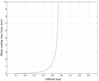
MrDr1 model. This waiting time shown in Figure 2.16 for N ™ .

40 BASICS OF PACKET SWITCHING

Fig. 2.16 The mean waiting time for input queuing with FIFO buffers for the limiting case for N s .

2.3.2 Output-Buffered Switches

With output queuing, cells are only buffered at outputs, at each of which a separate FIFO is maintained. Consider a particular Ži.e., tagged. output queue. Define the random variable A as the number of cell arrivals destined for the tagged output in a given time slot. Based on the same assumptions as in Section 2.3.1 on the arrivals, we have

Denote by Qm the number of cells in the tagged queue at the end of the mth time slot, and by Am the number of cell arrivals during the mth time slot. We have

42 BASICS OF PACKET SWITCHING

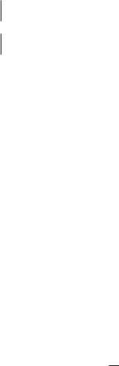
Fig. 2.17 The cell loss probability for output queuing as a function of the buffer size b and the switch size N, for offered loads Ža. p s 0.8 and Žb. p s 0.9.

Figure 2.17Ža. and Žb. show the cell loss probability for output queuing as

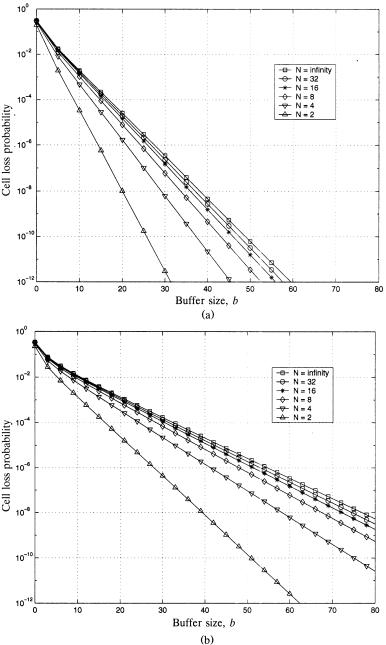
large N. The N ™ curve can be a close upper bound for finite N 32. Figure 2.18 shows the cell loss performance when N ™ against the output buffer size b for offered loads p varying from 0.70 to 0.95.

Output queuing achieves the optimal throughput delay performance. Cells are delayed unless it is unavoidable, when two or more cells arriving on different inputs are destined for the same output. With Little’s result, the

mean waiting time W can be obtained as follows:

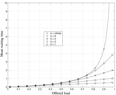
Figure 2.19 shows the numerical results for the mean waiting time as a function of the offered load p for N ™ and various values of the output buffer size b. When N ™ and b ™ , the mean waiting time is obtained from the MrDr1 queue as follows:

p

W s 2 Ž1 y p. .

Fig. 2.18 The cell loss probability for output queuing as a function of the buffer size b and offered loads varying from p s 0.70 to p s 0.95, for the limiting case of

N ™ .

44 BASICS OF PACKET SWITCHING

Fig. 2.19 The mean waiting time for output queuing as a function of the offered load p, for N ™ and output FIFO sizes varying from b s 1 to .

2.3.3 Completely Shared-Buffer Switches

With complete buffer sharing, all cells are stored in a common buffer shared

cell arrivals. Output queuing can be maintained logically with linked lists, so that no cells will be blocked from reaching idle outputs, and we still can achieve the optimal throughput delay performance, as with dedicated output queuing.

In the following, we will take a look at how this approach improves the cell loss performance. Denote by Qmi the number of cells destined for output i in the buffer at the end of the mth time slot. The total number of cells in the

where Aim is the number of cells addressed to output i that arrive during the mth time slot.

With a finite buffer size, cell arrivals may fill up the shared buffer, and the resulting buffer overflow makes Ž2.13. only an approximation. However, we